Generating a mass gap using Feynman diagrams in an
asymp-totically free theory
VenkiteshAyyar1and ShaileshChandrasekharan2,
1Department of Physics, University of Colorado at Boulder, Boulder CO 80309 2Department of Physics, Duke University, Durham NC 27708
Abstract.Using the example of a two dimensional four-fermion lattice field theory, we show that Feynman diagrams can generate a mass gap in a theory with massless fermions that interact via a marginally relevant coupling. We show this by introducing an infrared cutoffthat makes the perturbation series for the partition function convergent. We use a
Monte Carlo approach to sample sufficiently high orders of diagrams and thus expose the
presence of the mass gap.
1 Introduction
Asymptotically free quantum field theories are defined through a Gaussian fixed point with a marginally relevant coupling. This suggests that a non-perturbative approach based on an expan-sion in powers of some bare couplingU should be able to describe the physics quantitatively. Re-cently, Monte Carlo methods that sample bare weak coupling Feynman diagrams have emerged as a new way to extract non-perturbative physics in a variety of models [1–6]. Can such methods be ex-tended to asymptotically free theories like QCD? Setting aside complications due to gauge invariance, here we explore this question in a simple fermionic toy model in two dimensions. Similar questions have been raised recently and partially addressed within the context of the two dimensionalO(N) and U(N)×U(N) models in the largeNlimit [7,8]. Non-perturbative methods based on resurgence theory [9] and the bootstrap program have also addressed similar questions recently [10].
Naively, one would think that it is impossible to obtain the mass gap using a weak coupling diagrammatic approach, since the non-perturbative mass gap in the theory scales asM ∼e−β/U. The
essential singularity atU =0 would invalidate any perturbative approach. In this talk we argue that by regulating the ultraviolet and infrared divergences in a controllable way, it is possible to make the weak coupling series convergent at least in two dimensional four-fermion field theories like the Gross Neveu models that are known to be asymptotically free [11,12]. We consider an explicit example of the lattice model and show how Feynman diagrams generate the mass gap in this theory [13].
2 Lattice Model
The model we consider is constructed using reduced staggered fermions [14,15], whose action is given by
S(ψ) = 1 2
x,y,a
ψaxMx,yψay − U
x
ψ4xψ3xψ2xψ1x, (1)
whereMx,yis the free staggered fermion matrix
Mx,y =
1 2
α
ηα,xδx+α,yˆ −δx−α,yˆ , (2)
with the phase factorsη1,x=1,η2,x=(−1)x1. Note that there is only a single Grassmann valued field ψaxin the lattice action. The partition function of the model is given by
Z=Z0
[dψ] e−S(ψ) (3)
whereZ0is chosen so thatZ =1 in the free theory and the integration measure [dψ] is the propduct of [dψ1xdψ2xdψ3xdψ4x] on every sitex.
AtU=0 our lattice model describes four flavors of free massless (two-component) Dirac fermions in the continuum limit, which is reached by exploring physics at large length scales as compared to the lattice spacing. As a probe of the long distance physics we can take space-time to be a torus of side L(in lattice units) in each direction with anti-periodic boundary conditions. In two dimensions, a free fermion field is expected to have a mass dimension [ψax]=1/2. In our approach this can be seen from
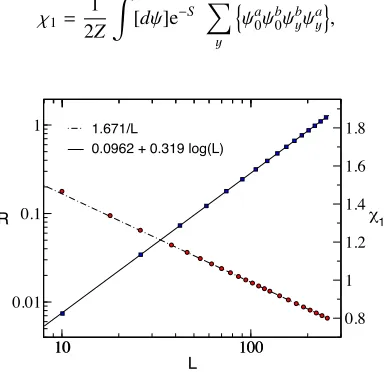
the scaling of the fermion propagatorGf(x, y)∼1/|x−y|for large separations. In Fig.1we plot the
scaling of the propagator at a separation of|x−y|=L/2 along one of the directions,R=Gf(0,L/2)
as a function ofL. As expected we findR∼1/L. In the same figure we also show the scaling of the susceptibility
χ1= 1 2Z
[dψ]e−S y
ψa0ψb0ψbyψay
, (4)
10 100
L
0.01 0.1 1
R
1.671/L
10 100
0.8 1 1.2 1.4 1.6 1.8
χ1
0.0962 + 0.319 log(L)
2 Lattice Model
The model we consider is constructed using reduced staggered fermions [14,15], whose action is given by
S(ψ) = 1 2
x,y,a
ψaxMx,yψay − U
x
ψ4xψ3xψ2xψ1x, (1)
whereMx,yis the free staggered fermion matrix
Mx,y =
1 2
α
ηα,xδx+α,yˆ −δx−α,yˆ , (2)
with the phase factorsη1,x=1,η2,x=(−1)x1. Note that there is only a single Grassmann valued field ψaxin the lattice action. The partition function of the model is given by
Z=Z0
[dψ] e−S(ψ) (3)
whereZ0is chosen so thatZ =1 in the free theory and the integration measure [dψ] is the propduct of [dψ1xdψ2xdψ3xdψ4x] on every sitex.
AtU=0 our lattice model describes four flavors of free massless (two-component) Dirac fermions in the continuum limit, which is reached by exploring physics at large length scales as compared to the lattice spacing. As a probe of the long distance physics we can take space-time to be a torus of side L(in lattice units) in each direction with anti-periodic boundary conditions. In two dimensions, a free fermion field is expected to have a mass dimension [ψax]=1/2. In our approach this can be seen from
the scaling of the fermion propagatorGf(x, y)∼1/|x−y|for large separations. In Fig.1we plot the
scaling of the propagator at a separation of|x−y|=L/2 along one of the directions,R=Gf(0,L/2)
as a function ofL. As expected we findR∼1/L. In the same figure we also show the scaling of the susceptibility
χ1= 1 2Z
[dψ]e−S y
ψa0ψb0ψbyψay
, (4) 10 100 L 0.01 0.1 1 R 1.671/L 10 100 0.8 1 1.2 1.4 1.6 1.8 χ1
0.0962 + 0.319 log(L)
Figure 1. The scaling of the fermion propagator at the mid point (R) and the susceptibility (χ1) as a function of Lin the free theory. This shows that the couplingUis perturbatively marginal as expected in the continuum.
as a function ofL. This susceptibility is naively dimensionless, but due to infrared singularities it is expected to diverge logarithmically with the lattice sizeL. This behaviour is consistent with the fact that the couplingUis marginal as expected from continuum perturbative power counting. We will see later that in factU is marginally relevant since an exponentially small mass gap is generated in this model whenU>0 due to asymptotic freedom as predicted originally by Gross and Neveu [11].
3 The Partition Function
Let us first expand the partition function of our model in powers of the coupling,
Z = Z0
[dψ] e−1
2ψTMψexUψx4ψ3xψ2xψ1x = Z0
[dψ] e−1
2ψTMψ x
1+Uψ4
xψ3xψ2xψ1x
= Z0
k
Uk
[x,k]
a
[dψa] e−12ψaxMx,yψayψa x1ψ
a x1...ψ
a xk
=
k
Ukz
k, (5)
where the coefficientszkcan be obtained as a sum over weights of all possible vertex configurations
[x;k] = {x1,x2, ...,xk}. Each configuration is an ordered set of k different lattice sites where the interactions occur and has the weight given by
Ω([x;k]) = Z0
a
[dψ]e−12ψxaMx,yψayψa x1ψ
a x2...ψ
a xk
4
= Pf(W([x;k])4, (6)
which is a sum over Feynman diagrams obtained through the regular Wick contractions. In the last step we have used the fact that for each flavor the sum over the diagrams is equal to the Pfaffian of ak×kmatrixW([x;k]), whose matrix elements are given by the free staggered fermion propagator Gf(xi,xj) between the sites in [x;k] [16]. SinceΩ([x;k]) is positive a Monte Carlo method can then
be used to sample the vertex configurations [x;k], which is distributed according to the probability distribution
Pk(U,[x;k]) = U k
Z(U)Ω([x;k]). (7)
Due to symmetries of the model only configurations [x;k] with an equal number of even and odd sites have non-zero weights, which implies that only even values ofkcontribute to the expansion in Eq.(5). Interestingly, the expansion in powers ofUis finite and completely convergent on a finite lattice. Since the maximum number of vertices that are allowed isL2 the partition functionZ is a polyno-mial. Our goal is to understand how the infrared divergences present in an asymptotically free theory manifest themselves in this polynomial. In order to gain some insight into the dominant terms in the expansion we define the probability distribution of vertices,Pk(U) = zkUk/Z(U). Note that Pk(U)
as the sum overPk(U,[x,k]) with a fixedkandUbut different locations of the vertices. While it is
difficult to computePk(U) analytically we can use Monte Carlo sampling to estimate it. In Fig.2(a)
we plotPk(U) atU =0.1 for different values ofL. Note that sectors with a large number of vertices
0 4 8 12
k
0 0.1 0.2 0.3
Pk
32 x 32
0 8 16 24 32 40
k 64 x 64
0 12 24 36 48 60
k 0
0.1 0.2 0.3
Pk 96 x 96
(a)
0 0.25 0.5 0.75 1 1.25 1.5 1.75 2 U
0 0.2 0.4 0.6 0.8 1
ρ(U)
L = 32
0 20 40 60 80 100 0
0.002 0.004
U = 0.1
(b)
Figure 2. (a) Probability distribution of vertices in the partition function as a function of the lattice size at U=0.1 forL=32,64 and 96. The average density of verticesρk=k/L2≈0.00267 remains constant in all the
three cases. (b) Plot of the density of verticesρ(U) as a function ofU. The inset shows the density atU=0.1 as
a function ofL. We see that the density of vertices remains the same asLincreases.
It is easy to understand why the average density of vertices is constant in the thermodynamic limit. From the point of view of statistical mechanics one expects the partition function of a two dimensional system to scale asZ=exp(f(U)L2), where f(U) is the free energy density. Interestingly, the average density of vertices is related tof(U) through the expression
ρ(U)=k
L2 = (U/L2)(∂lnZ(U)/∂U) = U(∂f(U)/∂U). (8) Sincef(U) is expected to be independent of the volume for sufficiently large volumes, we also expect ρ(U) to be independent of the volume.
10 20 30 40 50 60
L
0.11 0.12 0.13 0.14 0.15 0.16 0.17
fk
k=2 k=4
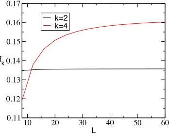
Figure 3. Plot of the perturbative coefficients f2and f4in the expansion of the free energy as a function ofL.
0 4 8 12
k
0 0.1 0.2 0.3
Pk
32 x 32
0 8 16 24 32 40
k 64 x 64
0 12 24 36 48 60
k 0
0.1 0.2 0.3
Pk 96 x 96
(a)
0 0.25 0.5 0.75 1 1.25 1.5 1.75 2 U
0 0.2 0.4 0.6 0.8 1
ρ(U)
L = 32
0 20 40 60 80 100 0
0.002 0.004
U = 0.1
(b)
Figure 2. (a) Probability distribution of vertices in the partition function as a function of the lattice size at U=0.1 forL=32,64 and 96. The average density of verticesρk=k/L2≈0.00267 remains constant in all the
three cases. (b) Plot of the density of verticesρ(U) as a function ofU. The inset shows the density atU=0.1 as
a function ofL. We see that the density of vertices remains the same asLincreases.
It is easy to understand why the average density of vertices is constant in the thermodynamic limit. From the point of view of statistical mechanics one expects the partition function of a two dimensional system to scale asZ =exp(f(U)L2), where f(U) is the free energy density. Interestingly, the average density of vertices is related tof(U) through the expression
ρ(U)= k
L2 = (U/L2)(∂lnZ(U)/∂U) = U(∂f(U)/∂U). (8) Since f(U) is expected to be independent of the volume for sufficiently large volumes, we also expect ρ(U) to be independent of the volume.
10 20 30 40 50 60
L
0.11 0.12 0.13 0.14 0.15 0.16 0.17
fk
k=2 k=4
Figure 3. Plot of the perturbative coefficients f2and f4in the expansion of the free energy as a function ofL.
The connection betweenZ(U) and f(U) is well known in diagrammatic perturbation theory; the former contains contributions from disconnected diagrams, while the latter gets contributions only
from connected diagrams. At a fixedLwe can expand f(U)= f2U2+ f4U4+...and find relations between the coefficients fk andzk. For example f2 = z2/L2 and f4 = (z4 −z22/2)/L2 and so on. From the discussion above we learn thatZ(U) contains no infrared divergences except for the usual factors of the volume, but we cannot rule out such divergences in the expansion of f(U). In general infrared divergences of perturbation theory appear in the fk’s as Lis increased. In our model such
divergences do not seem to appear at least in the first two terms f2and f4as can be seen in3, where these coefficients are plotted as functions ofL. This seems to be a special feature of our model due to its symmetries. Importantly, even if the fk’s contained divergences we can still extract f(U)
non-perturbatively through the integral
f(U) =
U
0 ρ(U)/U, (9)
if we can computeρ(U) non-perturbatively by summing over the distribution of vertices generated by the Monte Carlo method. The usual infrared divergences in perturbation theory disappear after this re-summation.
4 The Mass Gap
In order to see how Feynman diagrams generate the mass gap in our model we focus on the finite size susceptibilityχ1defined in (4). As we already pointed out earlier, in the free theoryχ1 diverges logarithmically for large values ofL(see Fig.1). However, if a mass gapMis generated we expect χ1to level offroughly aroundL ∼ M−1. The calculation ofχ1can also be expressed as a sum over Feynman diagrams through the relation,
χ1 =
y,k [x;k]
Γ0,y([x;k])Pk(U,[x;k])
(10)
whereΓ0,y([x;k]) is the ratio of two quantities. The numerator is the sum over all Feynman diagrams
with two fermion bilinear sourcesψa0ψb0 andψbyψay, the former located at the origin and the latter at y, in addition to the vertices [x;k] ={x1,x2, ...,xk}. The denominator isΩ([x;k]), i.e., the sum over Feynman diagrams without the sources. This ratio makesΓ0,y([x;k]) scale like a “connected”
Feyn-man diagram for large volumes since the factor that scales exponentially in the volume is cancelled between the numerator and the denominator.
In order to computeχ1we generate the vertex configurations [x;k] with probabilityPk(U,[x;k])
and then introduce sources, one chosen at a random lattice site which is defined as the origin and another at the site ywhich is moved sequentially through the lattice. We then compute χ1 using Eq. (10). In Fig.4(a) we plotχ1as a function ofLatU =0.3 and 0.4. Note that indeedχ1 begins to level offaroundL ∼128 atU =0.3 and aroundL∼32 atU=0.4, implying that a mass gap has been generated. The fact that it takes a substantially larger value ofLbeforeχ1levels offatU=0.3 as compared toU=0.4 is an indication thatMis decreasing rapidly. We also plot theU =0 results for comparison.
Statistically speaking this implies that for most vertex configurations [x;k] generated in the Monte Carlo sample,Γ0,y([x;k]) begins to decay exponentially for pointsyfar from the origin. This implies
8 16 32 64 128 L 0
1 2 3 4 5 6
χ1
U = 0.4 U = 0.3 U = 0.0
0.2 0.3 0.4 0.5 U
2 3 4 5 6
χ1 L = 128 L = 32
(a)
0 100 200 300 400 500 Monte Carlo Sweep
0 5 10 15 20
χ1
(b)
Figure 4. (a) Plot of the susceptibilityχ1as a function ofLforU=0,0.3 and 0.4 (left figure), and as a function ofUforL = 32 and 128 (right figure). For values ofLlarger thanM−1 (the inverse mass gap)χ1begins to saturate. For each value ofL, we can also define the mass scaleMb =L−1 defined at the location of the peak
U=Up. We see that roughlyM ∼ Mb. (b) Fluctuations ofχ1in a sample of 500 vertex configurations [x;k] generated consecutively during the Monte Carlo sampling. Rare but large fluctuations seem to be the remnant of infrared divergences.
(a)
16 32 64 128 256
L
0.2 0.3 0.4 0.5 0.6 0.7
Up
1.33/log(0.88 L)
16 32 64 128 256
L
0 2 4 6 8
χ1,p 1.77 log (0.20 L)
(b)
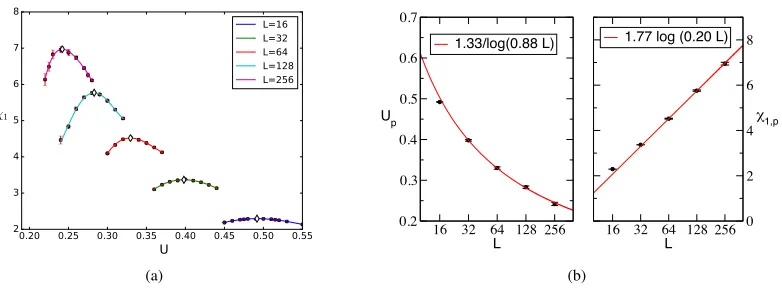
Figure 5. (a) Plot ofχ1as a function ofUfor different values ofL. The locations of the peak obtained by fitting the data to a smooth curve (quartic functions) are listed in Tab.1. (b) Plot ofUpandχ1,pas a function ofLand the fits to Eq.(11).
8 16 32 64 128 L 0
1 2 3 4 5 6
χ1
U = 0.4 U = 0.3 U = 0.0
0.2 0.3 0.4 0.5 U
2 3 4 5 6
χ1 L = 128 L = 32
(a)
0 100 200 300 400 500 Monte Carlo Sweep
0 5 10 15 20
χ1
(b)
Figure 4. (a) Plot of the susceptibilityχ1as a function ofLforU=0,0.3 and 0.4 (left figure), and as a function ofU forL =32 and 128 (right figure). For values ofLlarger thanM−1(the inverse mass gap)χ1 begins to saturate. For each value ofL, we can also define the mass scaleMb =L−1 defined at the location of the peak
U =Up. We see that roughlyM ∼ Mb. (b) Fluctuations ofχ1in a sample of 500 vertex configurations [x;k] generated consecutively during the Monte Carlo sampling. Rare but large fluctuations seem to be the remnant of infrared divergences.
(a)
16 32 64 128 256
L
0.2 0.3 0.4 0.5 0.6 0.7
Up
1.33/log(0.88 L)
16 32 64 128 256
L
0 2 4 6 8
χ1,p 1.77 log (0.20 L)
(b)
Figure 5. (a) Plot ofχ1as a function ofUfor different values ofL. The locations of the peak obtained by fitting the data to a smooth curve (quartic functions) are listed in Tab.1. (b) Plot ofUpandχ1,pas a function ofLand the fits to Eq.(11).
fluctuations in the Monte Carlo approach. We do see such rare fluctuations in our data. For example in Fig.4(b) we plot the fluctuations inχ1during a sample of the Monte Carlo time history forL=64 and U=0.4. As can be seen in Fig.4(a), for these parameters the susceptibility has already saturated to the valueχ1 ≈3.7. However, as Fig.4(b) shows there are still large but rare fluctuations inχ1that are five times larger. The fact that these divergent contributions are rare compared to finite contributions cannot be easily uncovered in usual perturbation theory.
For a quantitative analysis, instead of measuring the conventional mass gap we can define a slightly different mass scaleMbas follows. We first note that the susceptibilityχ1has a peak when it is plotted as a function ofU for every fixed value ofL. This behavior is clearly visible in the right figure of Fig.4(a) where we plotχ1as a function ofUatL=32 and 128. For a fixedLif the peak occurs at U =Up, we defineMb ≡ L−1as the non-perturbative mass scale generated atU =Up. Comparing the left and right figures in Fig.4(a) we see that our definition ofMbis also roughly consistent with
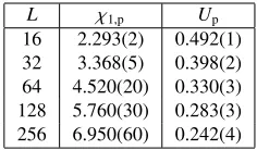
the value ofMobtained using the value ofLwhereχ1begins to level off. We have located the peaks at various lattice sizes accurately by fitting the data to quartic functions as shown in Fig.5(a). Table1
gives the values of the peak obtained through such a fit at different values ofL.
Table 1. Fit values forχ1,pandUpas a function ofL.
L χ1,p Up 16 2.293(2) 0.492(1) 32 3.368(5) 0.398(2) 64 4.520(20) 0.330(3) 128 5.760(30) 0.283(3) 256 6.950(60) 0.242(4)
If our theory is asymptotically free we expect thatMb= Λexp(−β/Up). Further, the peak value of the susceptibilityχ1,pis expected to grow logarithmically in the continuum limit. Thus, for sufficiently large values ofLwe expect
χ1,p = αlog(Λ1L), Up =log(Λβ
2L), (11)
In Fig.5(b) we show that our results are consistent with both these expectations. The parameters obtained from the fit to our data givesα=1.77(4),β=1.33(4),Λ1=0.20(1) andΛ2=0.88(9). It is usually difficult to matchβwith one loop perturbation theory since very large correlation lengths are needed [17]. On the other hand, qualitative exponential scaling of mass gaps as we show here, can be observed more easily [18].
5 Conclusions
References
[1] N.V. Prokof’ev, B.V. Svistunov, Phys. Rev. Lett.81, 2514 (1998) [2] N. Prokof’ev, B. Svistunov, Phys. Rev. Lett.99, 250201 (2007)
[3] M. Boninsegni, N.V. Prokof’ev, B.V. Svistunov, Phys. Rev. E74, 036701 (2006) [4] N.V. Prokof’ev, B.V. Svistunov, Phys. Rev. B77, 125101 (2008)
[5] E. Kozik, et.al., Europhys. Lett.90, 10004 (2010)
[6] G. Cohen, E. Gull, D.R. Reichman, A.J. Millis, Phys. Rev. Lett.115, 266802 (2015) [7] P.V. Buividovich, PoSLATTICE2015, 293 (2016)
[8] P.V. Buividovich, A. Davody (2017),arXiv:1705.03368
[9] A. Cherman, D. Dorigoni, G.V. Dunne, M. Unsal, Phys. Rev. Lett.112, 021601 (2014) [10] P. Orland, Phys. Rev.D90, 125038 (2014),1410.2627
[11] D.J. Gross, A. Neveu, Phys. Rev. D10, 3235 (1974) [12] E. Witten, Nuclear Physics B145, 110 (1978)
[13] V. Ayyar, S. Chandrasekharan (2017),arXiv:1709.06048 [14] H. Sharatchandra, H. Thun, P. Weisz, Nucl.Phys.B192, 205 (1981) [15] C. van den Doel, J. Smit, Nucl.Phys.B228, 122 (1983)