Comparative studies of the deformation techniques for the
singular-drift problem in the complex Langevin method
Yuta Ito1,⋆and Jun Nishimura1,2
1KEK Theory Center, High Energy Accelerator Research Organization, 1-1 Oho, Tsukuba, Ibaraki 305-0801, Japan
2Graduate University for Advanced Studies (SOKENDAI), 1-1 Oho, Tsukuba, Ibaraki 305-0801, Japan
Abstract.In application of the complex Langevin method to QCD at high density and low temperature, the singular-drift problem occurs due to the appearance of near-zero eigenvalues of the Dirac operator. In order to avoid this problem, we proposed to de-form the Dirac operator in such a way that the near-zero eigenvalues do not appear and to extrapolate the deformation parameter to zero from the available data points. Here we test three different types of deformation in a simple large-Nmatrix model, which under-goes an SSB due to the phase of the fermion determinant, and compare them to see the consistency with one another.
1 Introduction
When the action is complex, the integrand in the path integral cannot be regarded as the probability distribution. Therefore, the usual Monte Carlo simulations cannot be applied to such systems. A brute-force method is the so-called re-weighting method, but since the complex phase oscillates violently as the system size increases, it is difficult to evaluate the expectation values using this kind of method.
The complex Langevin method (CLM) [1,2] is a promising approach to this sign problem. It can be viewed as a complex extension of the stochastic quantization based on the Langevin equation. The idea of the CLM is to complexify the dynamical variables and to consider the holomorphic extension of the action and the observables. While the CLM works even in some systems that suffer from a
severe sign problem, it gives simply wrong results in the other cases. One of the recent developments concerns the conditions required for justification of the method. It was found that the probability distribution of the drift term has to fall offfaster than exponential [3]. There are two cases in which
this is not satisfied. One is the case in which the dynamical variables make long excursions into the imaginary direction [4]. The other is the case in which there is a non-vanishing probability that dynamical variables come close to the singularity of the drift term (the singular-drift problem) [5]. Another development was the invention of the gauge cooling technique [6], which made the CLM work in finite density QCD either at high temperature [7] or in the heavy dense limit [8].
At low temperature and high density, on the other hand, it is anticipated that the singular-drift problem occurs due to the appearance of near-zero eigenvalues of the Dirac operator. In ref. [9], we
proposed to avoid this problem by deforming the Dirac operator and extrapolating the deformation parameter to zero using only the reliable results obtained by the deformed model. We tested this idea in an SO(4)-symmetric matrix model with a Gaussian action and a complex fermion determinant, in which spontaneous breaking of the SO(4) symmetry is expected to occur due to the phase of the determinant [11]. This is also confirmed by explicit calculations based on the Gaussian expansion method (GEM) [12]. Applying the CLM to this model, we have found that the singular-drift prob-lem is actually severe because the fermionic part of the model is essentially an exactly “massless” system. Following the idea described above, we have found that the SO(4) symmetry of the origi-nal matrix model is broken spontaneously to SO(2) after extrapolating the deformation parameter to zero. The obtained results were indeed consistent with the prediction of the GEM albeit with small discrepancies.
There are, however, a few issues that remain to be addressed in this deformation technique. First the validity of the extrapolation relies on the assumption that there is no phase transition in the pa-rameter region in which the CLM does not work. Second it is not straightforward to estimate the systematic errors associated with the extrapolation. In order to address these issues, it is useful to think of various ways to deform the Dirac operator and to see how much the extrapolated results de-pend on the types of deformation. Here we investigate the aforementioned SO(4)-symmetric matrix model using three different types of deformed Dirac operator. We find that the results obtained by
these deformations are consistent with one another, which supports the validity and usefulness of the deformation technique as a solution to the singular-drift problem in the CLM.
The rest of this paper is organized as follows. In section2, we review the SO(4)-symmetric matrix model that we investigate in this work. In section3, we explain how we apply the CLM to the SO(4)-symmetric matrix model. In particular, we define three different types of deformation, each of which
can avoid the appearance of near-zero eigenvalues of the Dirac operator but with different ideas. In
section4, we present the results obtained by the three deformations and show that the results after extrapolating the deformation parameter are consistent with each other. We also conclude that the small discrepancies with the prediction from the GEM are due to the approximation used in the GEM. Section5is devoted to a summary and discussions.
2 Brief review of the SO(4)-symmetric matrix model
The SO(4)-symmetric matrix model investigated in this paper is defined by the partition function [11]
Z=
∫
dX (detD)Nfe−Sb, (1)
where the bosonic part of the action is given as
Sb =12N 4 ∑
µ=1
tr (Xµ)2. (2)
We have introducedN×NHermitian matricesXµ(µ=1, . . . ,4). The Dirac operatorDin eq. (1) is defined by
Diα,jβ= 4 ∑
µ=1
(Γµ)αβ(Xµ)i j. (3)
Here the 2×2 matricesΓµare the gamma matrices in 4d Euclidean space after Weyl projection defined by
Γµ=
proposed to avoid this problem by deforming the Dirac operator and extrapolating the deformation parameter to zero using only the reliable results obtained by the deformed model. We tested this idea in an SO(4)-symmetric matrix model with a Gaussian action and a complex fermion determinant, in which spontaneous breaking of the SO(4) symmetry is expected to occur due to the phase of the determinant [11]. This is also confirmed by explicit calculations based on the Gaussian expansion method (GEM) [12]. Applying the CLM to this model, we have found that the singular-drift prob-lem is actually severe because the fermionic part of the model is essentially an exactly “massless” system. Following the idea described above, we have found that the SO(4) symmetry of the origi-nal matrix model is broken spontaneously to SO(2) after extrapolating the deformation parameter to zero. The obtained results were indeed consistent with the prediction of the GEM albeit with small discrepancies.
There are, however, a few issues that remain to be addressed in this deformation technique. First the validity of the extrapolation relies on the assumption that there is no phase transition in the pa-rameter region in which the CLM does not work. Second it is not straightforward to estimate the systematic errors associated with the extrapolation. In order to address these issues, it is useful to think of various ways to deform the Dirac operator and to see how much the extrapolated results de-pend on the types of deformation. Here we investigate the aforementioned SO(4)-symmetric matrix model using three different types of deformed Dirac operator. We find that the results obtained by
these deformations are consistent with one another, which supports the validity and usefulness of the deformation technique as a solution to the singular-drift problem in the CLM.
The rest of this paper is organized as follows. In section2, we review the SO(4)-symmetric matrix model that we investigate in this work. In section3, we explain how we apply the CLM to the SO(4)-symmetric matrix model. In particular, we define three different types of deformation, each of which
can avoid the appearance of near-zero eigenvalues of the Dirac operator but with different ideas. In
section4, we present the results obtained by the three deformations and show that the results after extrapolating the deformation parameter are consistent with each other. We also conclude that the small discrepancies with the prediction from the GEM are due to the approximation used in the GEM. Section5is devoted to a summary and discussions.
2 Brief review of the SO(4)-symmetric matrix model
The SO(4)-symmetric matrix model investigated in this paper is defined by the partition function [11]
Z=
∫
dX (detD)Nfe−Sb, (1)
where the bosonic part of the action is given as
Sb=12N 4 ∑
µ=1
tr (Xµ)2. (2)
We have introducedN×NHermitian matricesXµ(µ=1, . . . ,4). The Dirac operatorDin eq. (1) is defined by
Diα,jβ = 4 ∑
µ=1
(Γµ)αβ(Xµ)i j. (3)
Here the 2×2 matricesΓµare the gamma matrices in 4d Euclidean space after Weyl projection defined by
Γµ=
i1σ2i forforµµ==4i=, 1,2,3, (4)
whereσi (i = 1,2,3) are the Pauli matrices. The model has an SO(4) symmetry, under which Xµ transforms as a vector.
The fermion determinant detDin (1) is complex in general. It was speculated that the SO(4) rotational symmetry of the model is spontaneously broken in the large-Nlimit with fixedr=Nf/N>0 due to the effect of the phase of the fermion determinant [11]. In the phase-quenched model, which is
defined by omitting the phase of the fermion determinant, the SSB was shown not to occur by Monte Carlo simulation [13]. We may therefore say that the SSB, if it really occurs, should be induced by the phase of the fermion determinant. Throughout this paper, we consider ther = 1 case, which
corresponds toNf =N.
In order to see the SSB, we introduce an SO(4)-breaking mass term
∆Sb=N
2ε 4 ∑
µ=1
mµtr (Xµ)2 (5)
in the action, where
m1<m2<m3 <m4, (6)
and we define the order parameters for the SSB by the expectation values of
λµ= 1
Ntr (Xµ)2, (7)
where no sum overµis taken. Due to the ordering (6), the expectation values obey
⟨λ1⟩>⟨λ2⟩>⟨λ3⟩>⟨λ4⟩ (8)
at finiteε. Taking the large-Nlimit and then sendingεto zero afterwards, the expectation values⟨λµ⟩ (µ=1,· · ·,4) may not take the same value. In that case, we can conclude that the SSB occurs. Here and henceforth, the parametersmµin the SO(4)-breaking term (5) are chosen as
(m1,m2,m3,m4)=(1,2,4,8). (9)
Explicit calculations based on the GEM were carried out assuming that the SO(4) symmetry is broken down either to SO(2) or to SO(3) [12]. Forr=1, the order parameters are given by
⟨λ1⟩=⟨λ2⟩ ∼2.1, ⟨λ3⟩ ∼1.0, ⟨λ4⟩ ∼0.8 for the SO(2) vacuum, (10) ⟨λ1⟩=⟨λ2⟩=⟨λ3⟩ ∼1.75, ⟨λ4⟩ ∼0.75 for the SO(3) vacuum. (11)
The free energy was calculated in each vacuum, and the SO(2)-symmetric vacuum was found to have the lower value.
3 Complex Langevin simulation with deformed Dirac operator
In this section, we explain how we apply the CLM to the SO(4)-symmetric matrix model (1). Includ-ing the symmetry breakInclud-ing term (5), we can write the partition function as
Z=
∫
-4 -3 -2 -1 0 1 2 3 4
-4 -3 -2 -1 0 1 2 3 4
Im
Re mf=0.6,ε=0.1, N=32
-4 -3 -2 -1 0 1 2 3 4
-4 -3 -2 -1 0 1 2 3 4
Im
Re mf=1.0,ε=0.1, N=32
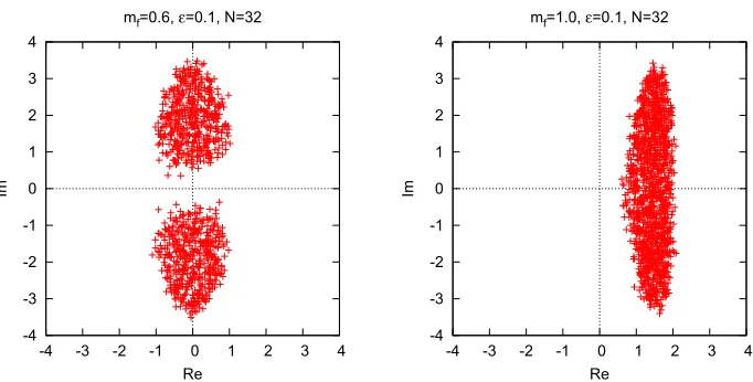
Figure 1.(Left) The scatter plot of the eigenvalues of the deformed Dirac operator (14) withε=0.1,mf =0.6 andN = 32. (Right) The scatter plot of the eigenvalues of the deformed Dirac operator (15) withε = 0.1,
mf =1.0 andN=32. In both plots, the configuration was obtained by simulating the corresponding deformed model.
The drift term that appears in the Langevin equation is given by
(vµ)i j= 1 w(X)
∂w(X) ∂(Xµ)ji
=−N (1+εmµ )
(Xµ)i j+Nf(D−1)iα,jβ(Γµ)βα (13)
as a function of the Hermitian matricesXµ. Note that the second term in (13) is not Hermitian in general corresponding to the fact that the fermion determinant is complex. Accordingly,Xµhas to be extended to general complex matrices as we solve the fictitious time evolution based on the Langevin equation1. The drift term (13) in the Langevin equation has to be defined for general complex matrices Xµby analytic continuation.
As we mentioned earlier, the singular-drift problem is associated with the appearance of near-zero eigenvalues of the Dirac operator D. Indeed we find that there are many eigenvalues close to zero forε ≤ 0.5, which implies that the extrapolation toε = 0 cannot be made reliably as it
stands. In order to circumvent this problem, we proposed to deform the Dirac operator [9]. Using this deformation technique, we have successfully shown in this matrix model that the SO(4) symmetry is broken spontaneously down to SO(2). However, the validity of the extrapolation relies on the assumption that there is no phase transition in the region that cannot be studied by the CLM. Also it is not straightforward to estimate the systematic error associated with the extrapolation. In order to address these important issues in the deformation technique, we consider three types of deformation of the Dirac operator and compare the result after extrapolations.
1In order to keep the matricesX
µas close to Hermitian as possible, we use the gauge cooling technique. Namely we
define the Hermiticity normNH=4N1 ∑4µ=1tr
[(
Xµ−Xµ†
) (
Xµ−Xµ†
)†]
,which measures the deviation ofXµfrom a Hermitian
-4 -3 -2 -1 0 1 2 3 4
-4 -3 -2 -1 0 1 2 3 4
Im
Re mf=0.6,ε=0.1, N=32
-4 -3 -2 -1 0 1 2 3 4
-4 -3 -2 -1 0 1 2 3 4
Im
Re mf=1.0,ε=0.1, N=32
Figure 1.(Left) The scatter plot of the eigenvalues of the deformed Dirac operator (14) withε=0.1,mf =0.6 andN = 32. (Right) The scatter plot of the eigenvalues of the deformed Dirac operator (15) withε = 0.1,
mf =1.0 andN=32. In both plots, the configuration was obtained by simulating the corresponding deformed model.
The drift term that appears in the Langevin equation is given by
(vµ)i j= 1 w(X)
∂w(X) ∂(Xµ)ji
=−N (1+εmµ )
(Xµ)i j+Nf(D−1)iα,jβ(Γµ)βα (13)
as a function of the Hermitian matricesXµ. Note that the second term in (13) is not Hermitian in general corresponding to the fact that the fermion determinant is complex. Accordingly,Xµhas to be extended to general complex matrices as we solve the fictitious time evolution based on the Langevin equation1. The drift term (13) in the Langevin equation has to be defined for general complex matrices Xµby analytic continuation.
As we mentioned earlier, the singular-drift problem is associated with the appearance of near-zero eigenvalues of the Dirac operator D. Indeed we find that there are many eigenvalues close to zero forε ≤ 0.5, which implies that the extrapolation toε = 0 cannot be made reliably as it
stands. In order to circumvent this problem, we proposed to deform the Dirac operator [9]. Using this deformation technique, we have successfully shown in this matrix model that the SO(4) symmetry is broken spontaneously down to SO(2). However, the validity of the extrapolation relies on the assumption that there is no phase transition in the region that cannot be studied by the CLM. Also it is not straightforward to estimate the systematic error associated with the extrapolation. In order to address these important issues in the deformation technique, we consider three types of deformation of the Dirac operator and compare the result after extrapolations.
1In order to keep the matricesX
µas close to Hermitian as possible, we use the gauge cooling technique. Namely we
define the Hermiticity normNH= 4N1 ∑4µ=1tr
[(
Xµ−Xµ†
) (
Xµ−Xµ†
)†]
,which measures the deviation ofXµfrom a Hermitian
configuration, and minimize this norm using SL(N,C) transformation after each Langevin step.
-4 -3 -2 -1 0 1 2 3 4
-4 -3 -2 -1 0 1 2 3 4
Im
Re z=0.5,ε=0.2, N=32
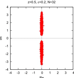
Figure 2. The scatter plot of the eigenvalues of the deformed Dirac operator (16) withε =0.2,z = 0.5 and
N=32. In this plot, the configuration was obtained by simulating the corresponding deformed model.
The first two types are the ones we have used in our previous work [9], which are defined by
D′
1A=Xµ⊗Γµ+mf1N⊗Γ3, (14)
D′
1B=Xµ⊗Γµ+mf1N⊗Γ4, (15) where we added the second term to the original Dirac operator (3) andmfis the deformation parameter. For sufficiently largemf, the second term changes the eigenvalue distribution of the Dirac operator in
such a way that there are no near-zero eigenvalues. In figure1, we plot the eigenvalue distribution of the deformed Dirac operators (14) and (15) obtained by simulating the corresponding deformed models. We find that the appearance of near-zero eigenvalues is avoided even forε=0.1. For a fixed mf, we can extrapolateεto zero using the results obtained in the large-Nlimit.
We can then extrapolate the deformation parametermf to zero to get the results for the original model. In this work we consider the third type of deformation, which is defined as
D′ 2=
3 ∑
i=1
Xi⊗Γi+zX4⊗Γ4, (16)
where we have introduced a deformation parameter z. The original model corresponds to z = 1
and the SO(4) symmetry is broken explicitly to SO(3) forz 1. Note that this deformed Dirac operatorD′
2becomes anti-Hermitian whenzis pure imaginary, in which case detD′2is real and there is no sign problem. In this sense the deformation parameterzmay be viewed as an analogue of the chemical potential in finite density QCD. The singular-drift problem is expected not to occur when |Rez|is small. In figure2, we plot the eigenvalue distribution of the deformed Dirac operators (16) obtained by simulating the corresponding deformed model. We find that the appearance of near-zero eigenvalues is avoided even forε=0.2. Note that forz=0, all the eigenvalues lie on the imaginary
0 0.1 0.2 0.3 0.4 0.5
0 0.2 0.4 0.6 0.8 1 1.2
ρµ
(
ε
=0,m
f
)
mf2
ρ1
ρ2
ρ3
ρ4
0 0.1 0.2 0.3 0.4 0.5
0 0.2 0.4 0.6 0.8 1 1.2
ρµ
(
ε
=0,m
f
)
mf2
ρ1
ρ2
ρ3
ρ4
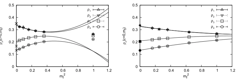
Figure 3.(Left) The ratioρµ(0,mf) obtained after taking the large-Nlimit and theε→0 limit in the deformed
model defined by (14) is plotted againstm2
f. The lines represent fits to the quadratic forma+bm2f +cm4f. The
crosses atmf=0 represent the prediction from the GEM. (Right) The ratioρµ(0,mf) obtained in the deformed
model defined by (15) is plotted againstm2
f. The lines represent fits to the quadratic forma+bm2f +cm4f. The
filled symbols atmf=0 represent the results obtained by the deformation (14).
zfor simplicity and see whether the SO(3) symmetry of the deformed model is spontaneously broken down to SO(2) as we increaseztowardsz=1. We also try to make an extrapolation toz=1.
4 Results
Before presenting our results, let us define the ratios
ρµ(ε,mf)=Nlim→∞ ⟨1
NtrX2µ ⟩
ε,mf
∑4 ν=1
⟨1 NtrX2ν
⟩ ε,mf
(17)
corresponding to the deformation (14) and similarly for the other deformations (15) and (16). This is motivated from the fact that the mass term (5) tends to make all the expectation values⟨λµ⟩ε,mfsmaller
than the value to be obtained in theε → 0 limit. By taking the ratio (17), the finiteεeffects are
canceled by the denominator, and the extrapolation toε=0 becomes easier.
In figure3(Left), we plot the ratioρµ(0,mf) after taking the large-Nlimit and theε → 0 limit againstm2
f for the deformation (14). The lines represent fits to the forma+bm2f+cm4f using the data for 0.2≤mf ≤0.6. By extrapolatingmf to 0, we obtain results for the original model. In figure3(Left), we also plot the prediction from the GEM with crosses atmf =0, which reveal certain discrepancies
from the results obtained by the extrapolation with the deformation (14).
In figure3(Right), we present a similar plot for the deformation (15). The lines represent fits to the forma+bm2f +cm4f using the data for 0.4≤mf ≤1.0. In the same figure, we also plot the results
obtained with the deformation (14) with filled symbols atmf = 0, which are found to be in good
agreement with the results obtained with the deformation (15). This implies that the discrepancies between our results and the prediction from the GEM are due to the approximation used in GEM.
0 0.1 0.2 0.3 0.4 0.5
0 0.2 0.4 0.6 0.8 1 1.2
ρµ ( ε =0,m f )
mf2
ρ1 ρ2 ρ3 ρ4 0 0.1 0.2 0.3 0.4 0.5
0 0.2 0.4 0.6 0.8 1 1.2
ρµ ( ε =0,m f )
mf2
ρ1
ρ2
ρ3
ρ4
Figure 3.(Left) The ratioρµ(0,mf) obtained after taking the large-Nlimit and theε→0 limit in the deformed
model defined by (14) is plotted againstm2
f. The lines represent fits to the quadratic forma+bm2f +cm4f. The
crosses atmf=0 represent the prediction from the GEM. (Right) The ratioρµ(0,mf) obtained in the deformed
model defined by (15) is plotted againstm2
f. The lines represent fits to the quadratic forma+bm2f +cm4f. The
filled symbols atmf=0 represent the results obtained by the deformation (14).
zfor simplicity and see whether the SO(3) symmetry of the deformed model is spontaneously broken down to SO(2) as we increaseztowardsz=1. We also try to make an extrapolation toz=1.
4 Results
Before presenting our results, let us define the ratios
ρµ(ε,mf)=Nlim→∞ ⟨1
NtrX2µ ⟩
ε,mf
∑4 ν=1
⟨1 NtrX2ν
⟩ ε,mf
(17)
corresponding to the deformation (14) and similarly for the other deformations (15) and (16). This is motivated from the fact that the mass term (5) tends to make all the expectation values⟨λµ⟩ε,mfsmaller
than the value to be obtained in theε → 0 limit. By taking the ratio (17), the finiteεeffects are
canceled by the denominator, and the extrapolation toε=0 becomes easier.
In figure3(Left), we plot the ratioρµ(0,mf) after taking the large-Nlimit and the ε → 0 limit againstm2
f for the deformation (14). The lines represent fits to the forma+bm2f+cm4f using the data for 0.2≤mf ≤0.6. By extrapolatingmf to 0, we obtain results for the original model. In figure3(Left), we also plot the prediction from the GEM with crosses atmf =0, which reveal certain discrepancies
from the results obtained by the extrapolation with the deformation (14).
In figure3(Right), we present a similar plot for the deformation (15). The lines represent fits to the forma+bm2f +cm4f using the data for 0.4≤mf ≤1.0. In the same figure, we also plot the results
obtained with the deformation (14) with filled symbols atmf = 0, which are found to be in good
agreement with the results obtained with the deformation (15). This implies that the discrepancies between our results and the prediction from the GEM are due to the approximation used in GEM.
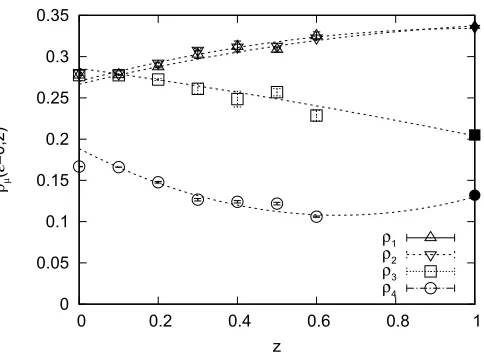
In figure4, we show our preliminary results for the deformation (16). We find that the SO(3) symmetry of the deformed model is spontaneously broken down to SO(2) forz ≳ 0.2. We have
0 0.05 0.1 0.15 0.2 0.25 0.3 0.35
0 0.2 0.4 0.6 0.8 1
ρµ ( ε =0,z) z ρ1 ρ2 ρ3 ρ4
Figure 4.The ratioρµ(0,z) obtained after taking the large-Nlimit and theε→0 limit in the deformed model
defined by (16) is plotted againstz. The filled symbols atz=1 represent the results obtained by the deformation (14). The dashed lines represent fits to the quadratic forma+bz+cz2using the data for 0.2≤z≤0.6 and the data points atz=1, which is obtained by deformation (14).
also attempted to make an extrapolation toz = 1 with the quadratic form a+bz+cz2 using the
data for 0.2 ≤z ≤ 0.6, but the uncertainties of our present data prevent us from making a reliable extrapolation at this stage. Here we would like to content ourselves with just checking the consistency with the deformation (14). For that purpose, we fit the data including the data points atz=1 obtained
by the deformation (14). The result of the fits looks reasonable as is shown in figure4with dashed lines. This suggests that it is possible improve the data so that we can make a reliable extrapolation without using the data points atz=1.
5 Summary and Discussions
In this article we discussed the deformation technique, which enables us to avoid the singular-drift problem that occurs in the CLM. We investigated the matrix model with a complex fermion deter-minant, in which the SO(4) symmetry is expected to be broken spontaneously down to SO(2) due to the effect of the phase of the fermion determinant. In order to avoid the singular-drift problem, we
deformed the Dirac operator in three different ways so that the appearance of near-zero eigenvalues
is suppressed. Our results suggest that the final results are independent of how we deform the Dirac operator. The deviations from the prediction by the GEM are therefore attributed to the approximation used in the GEM. The systematic errors associated with the extrapolation are considered to be smaller than these deviations. We hope that the insight gained in this work will be useful in applying the same technique to the complex Langevin analysis of finite density QCD at high density and low temperature [15].
to account for our four-dimensional space-time. On the other hand, the GEM [14] predicts that the SO(10) symmetry is broken down to SO(3) instead of SO(4). It would be interesting to address this issue extending the present work.
Acknowledgements
The authors would like to thank K.N. Anagnostopoulos, T. Azuma, K. Nagata, S.K. Papadoudis and S. Shimasaki for valuable discussions. Y. I. is supported by JICFuS. J. N. is supported in part by Grant-in-Aid for Scientific Research (No. 16H03988) from Japan Society for the Promotion of Science.
References
[1] G. Parisi,On complex probabilities, Phys. Lett. B131(1983) 393.
[2] J. R. Klauder,Coherent state Langevin equations for canonical quantum systems with applica-tions to the quantized Hall effect, Phys. Rev. A29(1984) 2036.
[3] K. Nagata, J. Nishimura and S. Shimasaki,Argument for justification of the complex Langevin method and the condition for correct convergence, Phys. Rev. D 94, no. 11, 114515 (2016) [arXiv:1606.07627 [hep-lat]].
[4] G. Aarts, E. Seiler and I. O. Stamatescu,The Complex Langevin method: When can it be trusted?, Phys. Rev. D81, 054508 (2010) [arXiv:0912.3360 [hep-lat]].
[5] J. Nishimura and S. Shimasaki,New insights into the problem with a singular drift term in the complex Langevin method, Phys. Rev. D92(2015) no.1, 011501 [arXiv:1504.08359 [hep-lat]]. [6] E. Seiler, D. Sexty and I. O. Stamatescu,Gauge cooling in complex Langevin for QCD with heavy
quarks, Phys. Lett. B723, 213 (2013) [arXiv:1211.3709 [hep-lat]].
[7] G. Aarts, E. Seiler, D. Sexty and I. O. Stamatescu, Simulating QCD at nonzero baryon den-sity to all orders in the hopping parameter expansion, Phys. Rev. D90(2014) no. 11, 114505 [arXiv:1408.3770 [hep-lat]].
[8] D. Sexty,Simulating full QCD at nonzero density using the complex Langevin equation, Phys. Lett. B729(2014) 108 [arXiv:1307.7748 [hep-lat]].
[9] Y. Ito and J. Nishimura,The complex Langevin analysis of spontaneous symmetry breaking in-duced by complex fermion determinant, JHEP1612, 009 (2016) [arXiv:1609.04501 [hep-lat]]. [10] N. Ishibashi, H. Kawai, Y. Kitazawa and A. Tsuchiya,A large N reduced model as superstring,
Nucl. Phys. B498(1997) 467 [hep-th/9612115].
[11] J. Nishimura, Exactly solvable matrix models for the dynamical generation of space-time in superstring theory, Phys. Rev. D65(2002) 105012 [hep-th/0108070].
[12] J. Nishimura, T. Okubo and F. Sugino, Gaussian expansion analysis of a matrix model with the spontaneous breakdown of rotational symmetry, Prog. Theor. Phys. 114 (2005) 487 [hep-th/0412194].
[13] K. N. Anagnostopoulos, T. Azuma and J. Nishimura,A practical solution to the sign problem in a matrix model for dynamical compactification, JHEP1110(2011) 126 [arXiv:1108.1534 [hep-lat]].