Available Online atwww.ijcsmc.com
International Journal of Computer Science and Mobile Computing
A Monthly Journal of Computer Science and Information Technology
ISSN 2320–088X
IMPACT FACTOR: 5.258
IJCSMC, Vol. 5, Issue. 5, May 2016, pg.221 – 230
Performance Comparison in
Digital Beamforming Using LMS,
RLS and D3LS Algorithms
Chirappanath B. Albert
*, Hao Chen
School of Engineering and Information Technology Charles Darwin University, Darwin, NT, 0909, Australia Email: [email protected] *, [email protected]Abstract - This paper presents a performance comparison of three different adaptive algorithms used in digital beamforming. These algorithms are used for the autonomous motion of the beams and for the cancellation of interferences. Discussion of using the least mean square, recursive least square and direct data domain least square algorithms for controlling the beam width, directivity, and sidelobe level are presented. The simulation results indicate that for least mean square and recursive mean square algorithms, the sidelobe level of the beam pattern remains the same for any number of antenna elements. The direct data domain least square algorithm enables us to achieve different sidelobes for same number of antenna elements. Based on the simulation results, an effective algorithm can be chosen to be used in a beamforming network according to the application. Direct data domain least square algorithm requires less time to determine the weights for digital beamforming compared to recursive least mean square algorithms which is has faster processing when compared to least mean square algorithm.
Keywords : “Direct Data Domain Least Square”, “Recursive Least Square”, “Least Mean Square”, “Digital Beamforming”, “Complex Weights”, “Windowing Functions”.
I. INTRODUCTION
the data from interferences [3]. In this approach, the covariance matrix obtained from the snapshots required heavy computation and large storage rooms. Unlike the statistical approach, deterministic algorithms or adaptive algorithms can be performed in real time, and were developed for the scenarios where the signal of interest is known as prior information. In this approach, the data is analysed from a single snapshot, and the interferences are cancelled by determining the weights without having to estimate the covariance matrix [4].
Digital beamforming technology progressed with the development of adaptive algorithms and architectures. The performance of a digital beamforming system is based on the number elements in an antenna array, the intermediate sampling frequency, the sampling rate, the signal frequency and the number of iterations required for converging, i.e. to obtain an error below a threshold level. Using least mean square (LMS) and recursive least mean square (RLS) algorithms to update the complex weights to form the beam and to acquire the signal of interest with minimum error have been investigated [5].
This paper presents the simulation results of using direct data domain least square (D3LS), recursive least mean square (RLS) and least mean square algorithm (LMS) in digital beamforming. The simulated beam patterns obtained from the three algorithms are compared.
II. DIGITAL BEAMFORMING
In digital beamforming, amplitude scaling and phase shifting are all done digitally with the aid of general purpose digital signal processors or dedicated beamforming chips. The signal received by each antenna element is digitised using an analog-to-digital converter (ADC). The signal received by the antenna array element is convoluted with the weighting functionthat is generated using the adaptive algorithms. The weighting functions are updated at every instance to reduce the error by the removal of the unwanted signals and the interferences from the signal of interest. The output obtained at the zero instant of time iscompared with and subtracted from the reference signal to obtain the error. A general expression for the signal along with the noise received by the kth antenna element of a digital beamforming network at the time t can be expressed as
k k k
X n u n jv n (1)
where uk(n) and vk(n) are the real and imaginary part of the complex baseband input signal respectively [7]. The
weighting function Wk(n) for the kth antenna is obtained using an adaptive algorithm and is given by
(2)
Where ak(n)and k(n)is the amplitude factor and the phase shift at the time t [7]. The signal at the output of the kth
antenna is given by
(3)
The error obtained at each instant of time is checked for the threshold value, if the error is above the threshold value, then the weighting functions are updated using the adaptive algorithms. The desired output is obtained when the error is reduced to reach the threshold level.
III. ADAPTIVE ALGORITHMS
The aim of incorporating an adaptive algorithm to a digital beamforming unit is to reduce the errors in the signal of interest and to increase the signal-to-noise ratio. The errors are reduced to a great extent by avoiding the unwanted signals, which is done by zero forcing and coherent cancelling of the signals. Zero forcing is a method where the antenna array units can adjust the direction of the nulls in a radiating pattern to the unwanted signals. According to this method the delays of the received signal are compensated by the process of equalising the delays. Coherent signal cancellation is performed by the method of destructive interference of the unwanted signal and the constructive interference of the required data signal of interest. With the aid of adaptive beamforming algorithms, the beam is made to adapt to the directions of signal of interest making the interferences and the unwanted signals to
sin
cos
k k k k
j u n v n
( )
cos
sin
k n Wk ak uk n k vk n k
X n
j k k k
n
W
n
a
n
e
cos( k
) sin(
)k n n j k
a
nA. Least Mean Square (LMS) Algorithm
The basic idea behind the LMS algorithm is that, it reduces the error content in the signal by squaring the expectation value of error signal and then finds out the total mean of all the error signals obtained from the each of the beamforming array units. The input is taken as X(n) and is composed of discrete set of values. The input is the convolute with the weighting functions W(n) to obtain the output. The output Y(n) is then compared with the reference signal d(n) and the error signal e(n) is produced. The input signal X(n) is represented by
( )
( ), (
1),...,
(
)
TX n
x n x n
X n k
(4)
0 1 1
( )
,
,...
k TW n
w w
w
(5)where k is the number of the antenna elements present in the array. The error signal is the difference between the output from the variable filter and the reference signal and is given by
T
e
n
d n
X
n
W
n
(6)where d(t) represents the reference signals, and T denotes conjugate transpose.[11] The equations (4) shows that the error signals are the difference between the output signals obtained and the reference signal. The error signal is then squared to reduce the errors as per the equation (5). LMS algorithm is an approximation of the steepest descent algorithm. It is represented by
(
1)
( )
( ( )
( )) ( )
W n
W n
y n
d n X n
(7)max
2
0
(8)where μ represents the step size and λmax represents the maximum eigenvalue of the autocorrelation matrix [11].
Least mean square algorithm is used to design a set of weighting coefficients that minimise the quadratic error signal and aid for fast converging [5]. The algorithm assumes smallest weightsin the initial condition and then updates by finding the gradient of the least mean square. If the mean square error is positive, we reduce the weights and if the mean square error is negative then the weights are increased [5].
B. Recursive Least Square (RLS) Algorithm
RLS is an algorithm with the same aim as that of LMS, where the input is considered to be deterministic. RLS has a memory that, it uses the past input together with current input. It shows that we depend on a variable filter and a self-updating weighting function in RLS algorithm [12]. The output of the filter is represented as
( )
( )
T( ).
y n
X n
W
n
(9)The error signal which is the difference of the obtained output and the desired output is feedback to the system, along with the input signal,
T
1
e
n
d
n
X
n W n
(10)The algorithm is initialized the values of weighting function to be zero W(n)=0. The input and the reference signal is also considered as zero X(n)=0,d(n)=0. We also consider P(n)=0 at the initial condition [12].
To decrease the influence of the input samples from the past, a weighting factor is used in RLS [5]. The weight update equation is given as
( )
(
1)
( )
( )
T( )
(
1)
where
K n
( )
is the gain coefficient and is given by1
1
(
1) ( )
( )
1
( )
T(
1) ( )
P n
X n
K n
X n P n
X n
(12)1 1
( ) [
(
1)] [
( ) ( )
T(
1)]
P n
P n
K n X n P n
(13)where λ is the forgetting factor, on which the the previous samples contribution depends [12].
C. Direct Data Domain Least Square (D3LS) Algorithm.
A direct data domain deterministic approach utilises a non-uniform array to adaptively estimate the signal strength of an incoming signal in the presence of strong jammers, clutter, and thermal noise. This method is based on choosing a weighted difference of neighbouring antenna outputs, based on the direction of arrival of the signal of interest; in such a way that only the unwanted components remain [13]. These unwanted signals are then nulled by adaptive weights. These weights are then used to estimate the signal strength for a set of sampling time instants [13]. Two main deterministic approaches are presented—one based on the solution of a generalized eigenvalue problem, the other based on the solution of a set of linear equations utilizing the conjugate gradient method. In this paper we focus on the eigenvalue method [13]. Here we consider a signal along with the presence of jammers, clutters and multipath with a centre frequency fs, the signal is extracted from the measure voltages of the antenna array.
The signal of interest, SOI, in phasor representation is
S j
S
S e
(14)
where, S is the complex signal of interest, |S| is magnitude of the same, and θSis the phase. It is assumed that the
signal is constant during the observation interval. The presence of the jammers with a carrier frequency same as that of SOI can be represented as
JAMMER
J
1
m sin
2
f
mn
m
sin
2
f
cn
c
]
(15)where fm is the modulating frequency, fc is the carrier frequency, m is the modulating index ,
J
represents theamplitude of the unwanted signal, ϕm and ϕc represents the modulating signal and interference phase respectively and
n being the time variable. Thermal noise contribution exists at each antenna element and is modeled as a real quantity, sampled from a uniform distribution between 0 and 1, and phase, again sampled from a uniform distribution between 0 and 2π.We can represent net signal as a combination of signal of interest, jammer, clutter and thermal noise [13].
If V is the output voltage of each antenna array element and S represents the incoming signal then
1 2
1 2
3 1
2
2 3 1
1 1
....
....
p p p m m p p p m mp p p
m m n
m m n m m
V
V
V
z
z
z
V
V
V
V
z
z
z
V
V
V
z
z
z
1 1 1
1 1 1
1 1 1 m m
S
(17)
where the matrix [S] is of unity rank, as we are dealing with a single signal of interest. The number of weighting functions used m, is given as
1
2
k
m
(18)The voltage level received at the kthantenna element is represented by
| |
sn n
k k
j k
v
z
S e
B
(19)
] }/ {2 [
z
j xksin s y cosk sk
e
(20)
where
V
kn is the net antenna output at time n andB
knrepresents the interference. The zk in the above equationindicates the contribution due to the progression of the signal phase front across the array elements. λ is the wavelength corresponding to the frequency of the SOI. Ψs is the angle of arrival of the SOI with respect to the x -axis. (xk, yk) indicate the coordinates of the kth antenna element in the plane [13]. The weights are so selected that the
unwanted signals are nulled out. The generalized eigenvalue equation is defined as
V
S
.
W
0
(21)The signal strength „α‟ is to estimate and is given by the generalized eigen value for the system. [W] is given by the generalized eigen vectors. The determinant of the equation is then equated to zero to determine „α‟ [13].
IV. SIMULATION RESULTS
We now present the simulation results to find the performance using D3LS, RLS and LMS algorithms. In the experiment, we took the D3LS algorithm for the estimation of the directivity, width and sidelobe level of the beam. Equations from (14) to equation (21) are used to get the simulation results by incorporating it to the adaptive algorithm. Different angle of arrival are taken into the consideration to find out the changes in the directivity, beamwidth and sidelobe level and a comparative table is made accordingly.
For the conventional algorithms using RLS and LMS, with the same features as above equations from (1) to equation (13) are taken into consideration and are incorporated into the adaptive algorithm in the for LMS and RLS respectively.
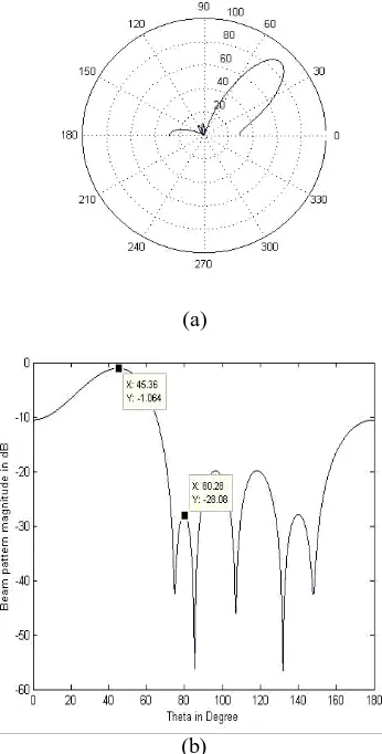
A: Radiation Pattern for Single Beam Using D3LS Algorithm:
(a)
(b)
Fig 1: (a) Radiation Pattern and (b) Frequency Domain for N=11and SOI=45
2. For the number of elements to be 21at 45ᵒ, directivity increased to 10.0dB beam width reduced to 15.4dB and the sidelobe level to-17dB
(b)
Fig 2: (a) Radiation Pattern and (b) Frequency Domain for N=21 and SOI=45
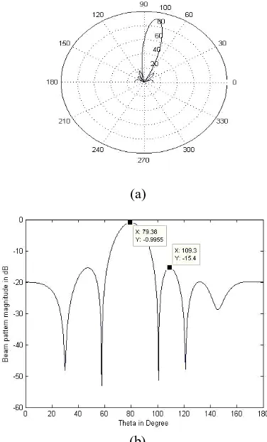
3. When the number of antenna array elements remains to be 11, and the SOI was changed to 80 the resultant beam had a directivity of 7.7 dB, beam width of 18.1 dB and a sidelobe level of -15dB when compared to that with SOI of 45showing with the increasing angle of arrival the beam gets narrower.
(a)
(b)
Fig 3: (a) Radiation Pattern and (b) Frequency Domain for N=11 and SOI=80
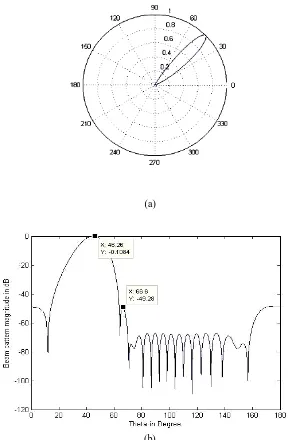
B: Radiation Pattern for Single Beam Using Conventional Algorithm
(a)
(b)
Fig 4: (a) Radiation Pattern and (b)Frequency Domain for N=11 and SOI=45
C: Comparative study of a single beam radiation pattern using D3LS with Conventional (LMS and RLS) Algorithms:
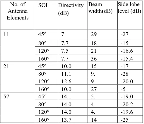
Table 1.Single beam radiation pattern at different angle of arrival with number antenna elements using D3LS
Table 2: Single beam radiation pattern at different angle of arrival with number antenna elements obtained using conventional algorithms (RLS and LMS)
Number of Elements
SOI Directivity (dB)
Beam Width(dB)
Side Lobe Level (dB)
11 45° 10.4 12.9 -13.0
80° 10.4 9.1 -13.0 120° 10.4 10.6 -13.0 160° 10.4 28.6 -13.1
21 45° 13.2 6.6 -13.5
80° 13.1 4.8 -13.2 120° 13.2 5.4 -13.2 160° 13.2 15.1 -13.2
57 45° 17.5 2.3 -13.2
80° 17.3 1.6 -13.3 120° 17.5 1.9 -13.3 160° 17.5 5.0 -13.2
Table 2 shows that under the influence of conventional algorithms, for any number of antenna elements from 11 to 57, the sidelobe level remains to be merely the same in the range of 13dB to 14dB. Directivity remains specific for each number of elements, and as the number of elements increase beam with always continue to decrease for a specific angle of arrival.
Inferences that are obtained from the simulation results are:
1. Beamwidth decreases as the beam moves from a minimum angle of 30° to 130° after which it start increasing.
2. The sidelobe level of the beams produced by the conventional algorithm is stable in the range of -13dB for any number of elements and angle of direction.
3. The directivity of the beam created by the conventional algorithm remains the same for any direction of arrival.
4. The D3LS algorithm has a smaller beamwidth when compare to the conventional algorithm, making it suitable foe point to point communication even in a short range.
5. The conventional algorithms better suits for the broadcasting applications. No. of
Antenna Elements
SOI Directivity (dB)
Beam width(dB)
Side lobe level (dB)
11 45° 7
. 4
29 .1
-27
80° 7.7 18
.1
-15 120° 7.5 21
.9
-16.6 160° 7.7 36
.2
-15.4
21 45° 10.0 15
.4
-17 80° 11.1 9.
9
-28 120° 12.6 9.
9
-20.0 160° 10.0 27
.7
-5
57 45° 14.1 5.
9
-19.0 80° 14.0 4.
1
-20.2 120° 14.0 4.
6
-19.6 160° 13.7 14
.0
6. D3LS algorithm exhibits instability with the changing direction of arrival, whereas the conventional algorithm is more stable.
7. Only a less amount of energy is wasted in the sidelobes caused by the D3LS algorithm, when compared to the conventional algorithm.
8. More data can be transmitted through the main beam created by the D3LS algorithm, when compared to the conventional algorithms with the same number of elements and direction of arrival.
V. CONCLUSION
Low directivity beams are used for the broadcasting communication whereas high directivity can be used for point to point communications. As the direction of arrival increases the directivity and beam width first decreases and then increases after 130ᵒ.The sidelobe level keeps decreasing with the increasing angle of arrival. The paper discusses only about one signal of interest while using the DDDLS algorithm, which can be worked upon with multiple signals of interest and along with multiple jammers being placed. The whole study is based upon the prior knowledge of direction of arrival (DOA) which can be also worked upon using different adaptive algorithms.
REFERENCES
[1] V. R. Lakshmi an G.S.N Raju, "Optimization of Raiation Patterns of Anteena Arrays," in PIERS Prooceing, Suhou, China, Septe,ber 2011.
[2] G.S.N Raju, Antennas an Propagation.: Pearson Education, 2005.
[3] J. Capon, “high-resolution frequency-wavenumber spectrum analysis,” Proceedings of the IEEE, vol. 57, no. 8, pp. 1408-1418, 1969..
[4] P. Zhang, J. Li, Z. Zhou , B. X. Hong, and Jian Bi, "A Robust Direct Data Domain Least Squares Beamforming with Sparse Constraint," Electromagnetic Resaerch C, vol. 43, pp. 53-65, 2013.
[5] D. Shashikumar and C. B. Albert, "Effect of Adaptive Filters and Windowing Functions on Bandwidth, Directivity and Time of igital Beam Forming," ACEEE, April 2013.
[6] L W Stutzman and A Thiele G, Antenna Theory and Design. NewYork, USA: John Wiley and Sons, 1981. [7] T. Hynes, "A Primer on Digital Beamforming," in Spectrum SIgnal Processing, March 1998.
[8] K. Max and W. Bernard, "A Variable Leaky LMS Adaptive Algorithm," ISL, Department of Electrical Engineering, Stanford University, 2004.
[9] K. Gurpreet and K. Guemeet , "Performance Evaluation of the Recursive Least Square Algorithm in Electronic Dispersion Compensation," pen Journel for Communication and SOftware, vol. 1, no. 2, August 2014.
[10] N. Srikanth ,M. C. Wicks T. K. Sarkar, "A Deterministic Direct Data Domain Approach to Signal Estimation Utilizing Nonuniform and Uniform 2-D Arrays," Digital Signal Processing 8, pp. 114-125, 1998.
[11] D.Bismor. “LMS Algorithm Step Size Adjustment for Fast Convergence” Archives of Acoustics, vol. 37, no. 1, pp. 31-40. 2012
[12] K.R.Borisagar and Dr. G. R. Kulkarni, “Simulation and Comparative Analysis of LMS and RLS Algorithms Using Real Time Speech Input Signal”, Global Journal of Researchers in Engineering, vol.10, no.5, pp.44. October 2010