Kasztelan, Christian (2010): Strongly Interacting Quantum Systems out of Equilibrium: Ultracold Quantum Gases and Magnetic Systems. Dissertation, LMU München: Fakultät für Physik

out of Equilibrium

Ultracold Quantum Gases and Magnetic Systems

Christian Kasztelan

Equilibrium

Ultracold Quantum Gases and Magnetic Systems

Christian Kasztelan

Dissertation

an der Fakult¨at f¨ur Theoretische Physik

der Ludwig–Maximilians–Universit¨at

M¨unchen

vorgelegt von

Christian Kasztelan

aus Gda´nsk (Danzig, Polen)

Zusammenfassung ix

Summary xi

Publication List xiii

1 Introduction and overview 1

1.1 Goals of this thesis . . . 3

1.2 Content of the thesis and outlook . . . 4

2 Matrix Product State, DMRG, Time evolution 7 2.1 Matrix Product States . . . 8

2.2 DMRG . . . 16

2.3 Time dependent DMRG methods . . . 21

2.3.1 Trotter Algorithm . . . 21

2.3.2 Krylov Algorithm . . . 23

2.3.3 Folding Algorithm . . . 25

3 Ultra Cold Gases 29 3.1 Bose Einstein Condensation . . . 30

3.1.1 BEC of an ideal gas . . . 31

3.1.2 Ultracold collisions . . . 32

3.1.3 BEC of a weakly interacting gas . . . 35

3.1.4 Thomas-Fermi approximation . . . 36

3.1.5 Recent development . . . 36

3.2 BEC in optical lattices . . . 38

3.2.1 Dipole force . . . 38

3.2.2 Optical potential . . . 39

3.2.3 Optical lattices . . . 39

3.2.4 Band structure . . . 40

3.2.5 Bose Hubbard Hamiltonian . . . 41

3.2.6 Recent development . . . 42

3.3.1 Time-of-flight and adiabatic measurement . . . 45

3.3.2 Noise correlations . . . 47

3.3.3 Recent development . . . 48

4 Magnetism, coherent many-particle dynamics, and relaxation with ultracold bosons in optical superlattices 51 4.1 Setup and model . . . 53

4.2 Effective model . . . 55

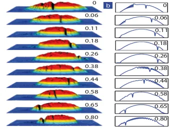
4.3 Time-evolution from the N´eel state . . . 57

4.3.1 Errors through experimental limitations in state preparation and measu-rement . . . 58

4.3.2 Symmetry between the ferromagnetic and the antiferromagnetic cases . . 60

4.3.3 Numerical method and parameters . . . 60

4.3.4 Site magnetization . . . 61

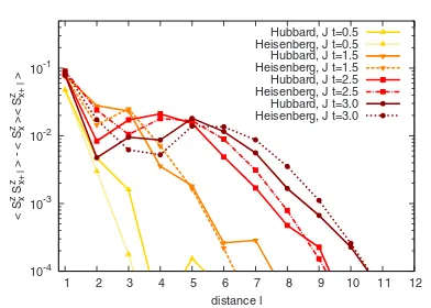
4.3.5 Correlation functions . . . 64

4.3.6 Momentum distribution and correlators . . . 64

4.4 Relaxation to steady states . . . 67

4.4.1 General features . . . 67

4.4.2 Relaxation for the Heisenberg magnet in mean field approximation . . . 68

4.5 Validity of the effective spin model . . . 71

4.6 Preparation of the antoferromagnetic groundstate by adiabatic evolution . . . 74

4.7 Conclusion . . . 76

5 Landau Zener dynamics on a ladder with ultra cold bosons 77 5.1 Mean field description . . . 78

5.1.1 Landau-Zener formula . . . 79

5.1.2 Extensions of the Landau-Zener formula . . . 80

5.2 Setup and model for the time-dependent DMRG calculations . . . 84

5.2.1 Numerical method and parameters . . . 85

5.3 Forward sweep . . . 85

5.4 Inverse sweep . . . 86

5.5 Time-evolution after quenches . . . 90

6 Entanglement and Decoherence of Multi-Qubit-Systems in external Baths 93 6.1 Quantifying Entanglement and Decoherence . . . 95

6.2 General entanglement law for entangled qubit pairs . . . 99

6.3 Few qubits in a general spin bath . . . 101

6.3.1 The two qubit case, Bell states . . . 103

6.3.2 The three and more qubit case, generalW- andGHZ-state . . . 108

6.3.3 Summary and outlook . . . 111

Der Hauptgegenstand dieser Arbeit ist die Untersuchung von Vielteilcheneffekten in stark kor-relierten eindimensionalen oder quasi-eindimensionalen Festk¨orpersystemen. Das charakteristi-sche an solchen Systemen sind ihre großen thermicharakteristi-schen und quantenmechanicharakteristi-schen Fluktuatio-nen. Da aufgrund dieser Eigenschaften ein Zugang mittels Molekularfeldmethoden oder auch st¨orungstheoretischer Methoden ausgeschlossen ist, k¨onnen solche Systeme in der Regel nur numerisch untersucht werden. Die Dichtematrix-Renormierungsgruppe (DMRG) ist eine ausge-reifte und gut verstandene Methode, die geeignet ist, um aussergew¨ohnlich große eindimensio-nale Systeme mit hoher Pr¨azision zu untersuchen. Diese ist 1992 von Steven White zun¨achst nur f¨ur statische Probleme entwickelt worden und wurde im Laufe der Zeit zu der zeitabh¨angigen DMRG erweitert, mit welcher sich auch Nichtgleichgewichtsszenarien erfolgreich untersuchen lassen.

In dieser Arbeit untersuche ich drei konzeptionell unterschiedliche Probleme, wobei ich gr¨oßtenteils die Krylov-Unterraum Variante der zeitabh¨angigen DMRG Methode benutze. Mei-ne Ergebnisse sind f¨ur k¨urzlich gemachte Experimente mit ultrakalten Atomgasen unmittelbar von Bedeutung. Diese Experimente sind unter anderem auch an der LMU in der Gruppe von Immanuel Bloch durchgef¨uhrt worden.

Modellen zu untersuchen. Es stellt sich heraus, dass die Relaxation beim Heisenberg Modell ¨uber eine Phasenmittelung geschieht, welche sich vollst¨andig vom Thermalisierungsprozess ¨uber St¨oße, welcher typisch f¨ur nicht-integrable Prozesse ist, unterscheidet.

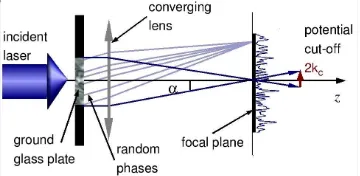
Im zweiten Teil meiner Arbeit untersuche ich die Erweiterung der urspr¨unglichen Landau-Zener Formel auf ein bosonisches Vielteilchensystem. Diese Formel gibt die Tunnelwahrschein-lichkeit zwischen den zwei Zust¨anden eines Zwei-Niveau Systems an, wobei die Energiediffe-renz zwischen diesen zwei Niveaus linear in der Zeit ver¨andert wird. In einem k¨urzlich reali-sierten Experiment wurde diese Fragestellung auf ein Vielteilchensystem ¨ubertragen, welches aus mehreren paarweise miteinander gekoppelten eindimensionalen Bose-Einstein Kondensaten besteht. Man hat festgestellt, dass die Kopplungst¨arke zwischen den Bose-Einstein Kondensaten und die Kopplung innerhalb der einzelnen Bose-Einstein Kondensate das urspr¨ungliche Landau-Zener Szenario stark modifizieren. Nach einer kurzen Einf¨uhrung in das Zwei-Niveau und das Drei-Niveau Landau-Zener Problem zeige ich die Resultate der Quantendynamik des mikrosko-pischen Modells und den Vergleich mit den experimentellen Ergebnissen. Dabei berechne ich sowohl die beiden m¨oglichen Landau-Zener Szenarien als auch die Zeitentwicklung zu einer fixen Energiedifferenz. Letzteres kann, vorausgesetzt die Anfangsteilchendichte ist ausreichend hoch, dazu benutzt werden, um einen quasi-thermalisierten Zustand mit einer beliebigen Tempe-ratur zu erzeugen.

The main topic of this thesis is the study of many-body effects in strongly correlated one- or quasi one-dimensional condensed matter systems. These systems are characterized by strong quantum and thermal fluctuations, which make mean-field methods fail and demand for a fully numerical approach. Fortunately, a numerical method exist, which allows to treat unusually large one -dimensional system at very high precision. This method is the density-matrix renormalization group method (DMRG), introduced by Steve White in 1992. Originally limited to the study of static problems, time-dependent DMRG has been developed allowing one to investigate non-equilibrium phenomena in quantum mechanics.

In this thesis I present the solution of three conceptionally different problems, which have been addressed using mostly the Krylov-subspace version of the time-dependent DMRG. My findings are directly relevant to recent experiments with ultracold atoms, also carried out at LMU in the group of Prof. Bloch.

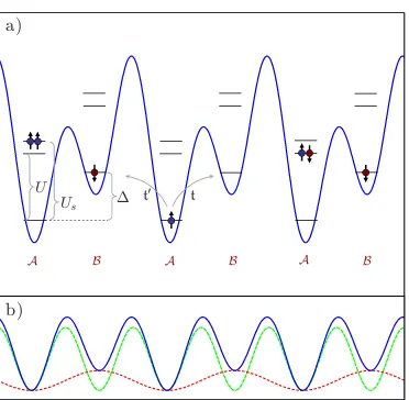
The first project aims the ultimate goal of atoms in optical lattices, namely, the possibility to act as a quantum simulator of more complicated condensed matter system. The underline idea is to simulate a magnetic model using ultracold bosonic atoms of two different hyperfine states in an optical superlattice. The system, which is captured by a two-species Bose-Hubbard model, realizes in a certain parameter range the physics of a spin-1/2 Heisenberg chain, where the spin exchange constant is given by second order processes. Tuning of the superlattice parameters allows one to controlling the effect of fast first order processes versus the slower second order ones. The analysis is motivated by recent experiments, where coherent two-particle dynamics with ultracold bosonic atoms in isolated double wells were detected. My project investigates the coherent many-particle dynamics, which takes place after coupling the double well. I provide the theoretical background for the next step, the observation of coherent many-particle dynam-ics after coupling the double wells. The tunability between the Bose-Hubbard model and the Heisenberg model in this setup could be used to study experimentally the differences in equi-libration processes for non-integrable and Bethe ansatz integrable models. It turns out that the relaxation in the Heisenberg model is connected to a phase averaging effect, which is in contrast to the typical scattering driven thermalization in nonintegrable models

During the course of the work for this thesis several articles have been published or made avail-able as preprints on arxiv.org.

• T. Konrad, F. de Melo, M. Tiersch, C. Kasztelan, A. Arag˜ao, and A. Buchleitner:Evolution equation for quantum entanglement,Nature Physics4, 99 - 102 (2008)

• T. Barthel, C. Kasztelan, I.P. McCulloch, and U. Schollw¨ock: Magnetism, coherent many-particle dynamics, and relaxation with ultracold bosons in optical superlattices, Phys.

Rev. A79, 053627 (2009)

Introduction and overview

With the first realization of Bose-Einstein condensation in dilute atomic gases in 1995 [10, 75, 42] a new and very dynamic field of physics emerged. Spectacular experiments with atomic Bose-Einstein condensates have demonstrated the remarkable wave-like nature of this new form of matter. Similar to the emitted light of a laser, which is a perfect realization of a classical electromagnetic wave, a Bose-Einstein condensate can be considered as the perfect realization of a classical matter wave.

The first generation of experiments with Bose-Einstein condensates focused on the coher-ence properties of these weakly-interacting superfluids. Some of the most important examples are the observation of interference between two overlapping condensates [14], of long-range phase coherence [39], and of quantized vortices and vortex lattices [1]. All of these phenom-ena can be explained by introducing a so-called macroscopic wave function or order parameter, which reduces the full many-body problem to a nonlinear single particle problem governed by the Gross-Pitaevskii equation for bosons or the Ginzburg-Landau theory for fermions.

Only a few years after the first realization of the BEC two other developments have cre-ated much attention among physicists with a background in condensed matter physics, nuclear physics and quantum information science. One is the ability to tune the interaction strength between atoms by means of so-called Feshbach resonances [64, 143], allowing one to enter the strongly interaction regime [302]. The other is the possibility to load ultracold quantum gases into optical lattices [118]. This technique allows to create the perfect periodic structure of arbitrary dimension and tunable tunneling rates. The combination of these two revolutionary techniques allows experimentalists to use cold atoms as quantum simulators, at first advocated by Richard P. Feynmann [99]. The quantum simulator is a highly controllable quantum system which is used to simulate the dynamical behaviour of another more complex quantum system [99]. An optical lattice offers remarkably clean access to a particular Hamiltonian and thereby serves as a model system for testing fundamental theoretical concepts and examples of quantum many-body effects.

particles must be transformed into a collective one, leading to a very special universality class for interacting quantum systems, known as Luttinger liquids [181]. Moreover, in one dimension quantum and thermal fluctuations are pushed to a maximum. This provides a severe limitation to mean-field approaches and fully numerical methods are generally needed to understand these physical systems.

Fortunately, in recent years a new numerical exact method, which goes under the name of density-matrix renormalization group (DMRG), allows one to treat unusually large one-dimensional systems at very high precision[242]. Only one decade after the initial DMRG formulation, given in 1992 by Steve White[284], and originally limited to the study of static problems, time-dependent renormalization group techniques have been developed, provide a interesting link between quantum information theory and computational condensed matter physics. This allows one to investigate quantum-many-body systems out of equilibrium, making DMRG a necessary tool to describe current experiments with ultra cold atoms in optical lattices [57].

Optical latices provide a flexible tool for probing fundamental condensed physics [37, 38], as well as finding applications in quantum optics [144, 175] and quantum information processing [43, 45, 38]. The clear realizations of many Hamiltonians and the high-tunability of the inter-nal parameters allow the creation of many different scenarios, which go beyond those currently achievable in typical condensed-matter physics systems [175]. One can create exotic many-body states [224], which are initially entangled [22] or states with a desired local density [260] as well as systems consisting of different types of bosons or fermions or mixtures between them [204]. By changing the lattice parameters or the whole lattice structure during an experiment it is possible to study exotic phase transitions [118, 128], transport phenomena [281] or non-equilibrium relaxation processes [157, 138] which have been so far unknown, or far from being fully understood.

A fundamental problem in quantum mechanics is the study of relaxation phenomena which occur in system coupled to an environment (open system). Closed systems, which are described by a pure wave function [44], can never relax on a global scale, since their total energy or sim-ilar conserved quantities remain constant throughout the whole time-evolution [101]. However, different subsystems of the total system can exchange energy or particles among each other and can therefore relax [24, 66]. These subsystems are simply open systems with respect to the rest of the total system, which acts as an environment. Beside the pure observation of relaxation, it remains an open question, how relaxation occurs in detail and what is the final relaxed state.

sub-systems stay in contact with each other the more entanglement will be created. Meanwhile, the observer becomes more and more ignorant until he makes a measurement on the system. In con-trast to a situation before turning on the spin-flips, a measurement now increases his amount of information about the system.

It is important to say that entanglement is not only a by-product of many-body quantum theory, as it is currently used as the key resource for many applications in quantum engineering [112, 139], like e.g. quantum communication [113] or quantum computing [82]. In a typical scenario one prepares a system consisting of few entangled particles, e.g. spin states, which are used later as the carrier of of some quantum information protocol [41, 250]. Since it is in general impossible to isolate this small system from some environment one will encounter all disadvantages of an open system here. As the entanglement between the system and the environment growths the valuable initial few-body entanglement in the system will decrease [163]. Thus, one observes also here a kind of redistribution of the quantity entanglement which comes along with the redistribution of the spins which have been entangled at the beginning.

1.1

Goals of this thesis

The aim of this thesis is the investigation of different many-body phenomena and relaxation physics of quantum many-particle lattice systems which are made either of interacting bosons moving in a lattice or, similarly, interacting spins that are localized on the sites of a quasi one-dimensional lattice. The here presented work is, mostly, strongly related to experiments with ultra cold atoms in optical lattices. With the help of the time-dependent DMRG method and, wherever it was possible or useful, other analytical calculations I have tried to:

(i) explain the experimentally observed quantum phenomena in one-dimensional atomic sys-tems. It turns out that very simple questions in quantum mechanics, which has been stated and already solved several decades ago, become fascinating again when put in the context of strongly interacting many-body quantum system. Due to the complexity of the new problems there is of-ten not even a simple picture which could explain the observed behaviour to entire satisfaction. This is in particular true for non-static problems. Despite the possibility to elaborate an an-swer analytically, e.g. using a mean-field approach, a precise analysis is only possible using the time-dependent DMRG method.

(ii) elaborate theoretical proposal for new and feasible experiments. Numerical analysis helps indeed to find the best parameter regime at which the desired many-body quantum effects are more visible but under the experimental constraints. Here the main purpose is to provide a complete physical picture of the relaxation process of some highly perturbed quantum state to a steady state in the long time limit.

1.2

Content of the thesis and outlook

The thesis is organized as follows. The first part consisting of two chapters, in which I introduce the DMRG method and in which I give an overview about the field of ultracold atoms in optical lattices, is followed by a second part in which I analyse three concrete problems.

Chapter 2 I give a summary of the density-matrix renormalization group methods in terms of the matrix product state (MPS) description. After introducing the MPS I explain all the necessary tools which are relevant for a successful implementation of a ground state and time-dependent DMRG method. In order make this preamble more readable, in particular for newcomers in the field of DMRG, I visualise most of the steps using also a simple pictorial language. In particular I present the two mostly used time-evolution methods, namely the Suzuki-Trotter and the Krylov-subspace method. I also provide a detailed formulation of a recently proposed time-evolution method, the so-called folding algorithm.

In Chapter 3 I give an overview on the topic of ultracold gases in optical lattices. In the first part I derive the so-called Gross-Pitaevskii equation for a weakly interacting Bose-Einstein condensate, which allows one to investigate coherent phenomena in ultra cold bosonic gases or macroscopic coherent phenomena. Moreover, I introduce the concepts of ultracold collisions and Feshbach resonances and provide the most important experimental quantities in the so-called Thomas-Fermi limit. In the second part I present the concept of optical lattices and derive the Bose-Hubbard Hamiltonian, which is the simplest model of strong correlated systems. The third and last part describes briefly the most common measurement techniques in optical lattices. I close each of the three parts by an up-to-date overview about the recent development.

In the second part of my thesis I present my results that follow from three different projects. The first two projects have been elaborated in collaboration between the theoretical group of Ulrich Schollw¨ock and the ultracold atoms group of Immanuel Bloch.

In 1932 L. Landau and C. Zener [170, 297] have derived a formula for the transition probabil-ity between the two states of a quantum mechanical two-level system, where the offset between the two levels is varying linearly in time. In Chapter 5 I investigate a many-body generalization of this original Landau-Zener scenario based on a recent experiment [57]. Here, the concept of the two-level system is extended to a system of pairwise tunnel-coupled one-dimensional Bose liquids with an time-dependent offset between the tubes. It turns out that the original Landau-Zener picture can be strongly modified by increasing the infratube and the intertube interactions. A particularly striking result is the breakdown of adiabaticity observed in the inverse sweep, which means that the initially filled tube is the one with higher energy. Contrary to the two-level model it turns out that in the many-body case slower sweeps lead to a lower transfer efficiency. Using the time-dependent DMRG I can qualitatively reproduce the experimental observations for the groundstate sweep as well as for the inverse sweep scenario. Moreover, I monitor the time-evolution of important quantities, e.g. momentum distribution or energies, in order to get a complete picture behind the breakdown. Additionally, I study the time-evolution after sud-den quenches of the energy offset. First of all, the quenches give a stroboscopic picture of the sweeps and reduce simultaneously the parameter space, and thus the complexity of the scenario. Second, it turns out that for sufficiently large initial density quenches can be efficiently used to create quasi-thermal states of arbitrary temperatures. The simplicity of the protocol allows for an easy experimental realization of these thermal states. After a introduction to the two-level and the three-level Landau-Zener problem I present my result for the quantum dynamics of the microscopic model and the comparison to the experimental results. I calculate the two possible Landau-Zener scenarios as well as the time-evolution after sudden quenches of the energy offset. A major finding is that for sufficiently large initial density quenches can be efficiently used to create quasi-thermal states of arbitrary temperatures.

Matrix Product State, DMRG, Time

evolution

Strongly correlated, low-dimensional quantum systems exhibit many extraordinary effects of modern many-body physics. Indeed such one- or two-dimensional structures are not exotic but have been found and studied often in nature. More recently, the advent of highly controlled and tunable strongly interacting ultracold atoms in optical lattices has added an entirely new direction to this field [38].

Now these kind systems are, both analytically and numerically, very hard to study. Exact solutions have been found only in some particular cases, e.g. by the Bethe ansatz in one di-mension. Moreover due to the strong interactions in such systems it is not possible to apply perturbation theories. Field theoretical approaches make many severe approximations and need to be additionally validated by numerical methods.

Fortunately, powerful numerical methods has been developed to study strong correlated low-dimensional systems . It was in 1992 when Steve White [283][284] has invented the density-matrix renormalization group (DMRG) method, which turned out to be one the most powerful methods for one-dimensional systems [242]. At the beginning it was only possible to study static properties (energy, order parameters,n-point correlation functions) of low-lying eigenstates, in particular the ground states. The method has been improved constantly becoming also a powerful tool to the study of dynamic properties of eigenstates, e.g. dynamical structure functions or frequency-dependent conductivities [165] [146], as well as the time-evolution of non-eigenstates under time-dependent and time-independent Hamiltonians [70] [285].

2.1

Matrix Product States

Considering a system with a finite system lengthL, e.g. an (anisotropic) Heisenberg antiferro-magnetic spin chain with an additional antiferro-magnetic field,

ˆ

H=

L−1

∑

J

2 S

+ i S

− i+1+S

− i S

+ i+1

+JzSz_iSz_i+1− L

∑

hSz_i. (2.1)

For a sufficient largeLit will be impossible to find an exact solution with, e.g., exact diagonal-ization methods. The reason for that is an exponential growth of the Hilbert space dimension with the system length. For a chain of spin-1₂ particles, with a local state dimensiond=2, the Hilbert space growth as dL=2L. Now it turns out that in many situations the relevant physics can be encoded in a much smaller effective Hilbert space using a parametrization provided by matrix product states.

In order to avoid exponential state space growth I assume an upper bound DdL for the state dimension. Once state dimension grows aboveD, state space has to be truncated down by some procedure. Now imagine that the state is sufficiently large and one therefore has to find a D-dimensional effective basis to describe it. In a first step I divide the system of the above Hamiltonian cutting it in three parts at some site l. The state can then be written as a linear combination of the tensor product between a left block{|a_l−1i}(sites 1, ...,l−1), the local spin state{|σli}at sitel, and a right block{|al+1i}(sitesl+1, ...,L)

|Ψi=

_∑

al−1

∑

σl

∑

ha_l−1σl|ali|al−1i|σli|al+1i, (2.2)

with|a_libeing the basis state for the left block together with the local spin state.

Introducing nowdmatricesAσ _{of dimension (D×D) each}1_{, I can rewrite the above equation} as

|Ψi=

_∑

al−1

∑

σl

∑

Aσl

al−1al|al−1i|σli|al+1i, (2.3)

whereAσl

al−1al =hal−1σl|aliis an arbitrary rank-3 tensor, as depicted in Fig.(2.1). The advantage

of the matrix notation is that it allows for a simple recursion formula to repeat this step for the left|a_l−1iblock

|Ψi=

_∑

al−1

∑

σl

∑

Aσl

al−1,al|al−1i|σli|al+1i

=

_∑

al−1,al−2

∑

σl−1,σl

∑

Aσl−1

al−2,al−1A σl

al−1,al|al−2i|σl−1i|σli|al+1i

=

_∑

a1,...,al−1

∑

σ1,..,σl

∑

Aσ1_1,a

1A σ2

a1,a2...A σl

al−1,al|σ1i|σ2i...|σli|al+1i. (2.4)

σi

ai₋1 ai

Aσi

ai−1,ai = |Ψ�

Aσ1_Aσ2 _Aσ3 _AσL

· · ·

· · ·

Figure 2.1: Matrix product state representation. The left figure shows the graphical representation of a singleAσi -tensor with an horizontal leg denotingσithe physical and two vertical legs denotingai−1andaithe row and column index respectively. The graphical representation of the whole matrix product state can be seen on the right.

Repeating the same procedure for the, so far, unchanged right block|a_l+1iI obtain

|Ψi=

_∑

ai

∑

1A σ2

a1,a2...A σl al−1,alA

σl+1

al,al+1...A σL

aL−1,aL|σ1i|σ2i...|σli|σl+1i...|σLi, (2.5) which in a more general way can be written as

|Ψi=

_∑

σ1,...,σi

Tr(Aσ1_...AσL_)|σ

1i...|σLi. (2.6)

Throughout out this chapter, only systems with open boundary conditions are considered. In this case the outer left matrices, Aσ1_{, and the outer right ones, A}σL_{, have the dimension 1}×_{d and} respectivelyd×12. Hence the trace becomes trivial and can be omitted

|Ψi=

_∑

σ1,...,σi

Aσ1_...AσL_|σ

1i...|σLi. (2.7)

Up to now I have introduced the matrix product state by adding piecewise one lattice site from a right block to the left block of the system which make the matrix product state growing from left to right. There are no particular constraints on the matricesAσ _{except that their dimensions}

must match appropriately. However, for certain operations, like the calculation of expectation values or the compressing of a matrix product state, to simplify, I demand that the chosen basis states for each block length are orthonormal to each other. If I assume the growth from left to right I obtain (for each left block) the condition

δ_a0

lal =ha 0

l|ali=

∑

∑

∑

σl Aσl†

a0_l−1,a0_lA

σl

al−1,al =

∑

(Aσl†_Aσl₎

a0_l,al. (2.8)

The above result can be summarized in a left-normalization condition (and similarly in right-normalization condition, assuming a growth form right to left)

∑

σ

Aσ†_Aσ _{=I left-normalization (2.9)}

∑

σ

Aσ_Aσ†_{=I right-normalization (2.10)}

In the following part I will show how to calculate, the overlap, expectation values, correlators in the matrix product state language.

Overlaps

As a first example of the advantage of MPS formulation I calculate the overlap between the two states|ψiand|φi, as depicted in Fig.(2.2). In order to avoid confusion I choseAto be the tensors

of|ψiandBtensors for|φi. Taking the adjoint of|φithe overlap reads

hφ|ψi=

_∑

σ

Bσ1∗...BσL∗_Aσ1_...AσL_{. (2.11)}

I would like to keep the above product structure between matrices, which is less complicated than a triple sum which includes the indicesai. Apparently, theBand theAare not in the right order. Fortunately transposing the whole product(Bσ1∗_...BσL∗₎T _{is all one has to do in order to} keep a product structure of matrices, but now in an order which makes the calculation much less demanding(CD)T =DTCT)

hφ|ψi=

_∑

σ

BσL†_...Bσ1†_Aσ1_...AσL_{. (2.12)}

If one decides to contract first over the matrix indices and then over the physical indices, he would have to sum overd_L strings of matrix multiplications. But this approach is exponentially costly. Now it turns out, that it is much easier to first sum over the physical index σ to obtain

a matrix (so matrix multiplication can be used), which in the next step is calculated as product between three matrices. Following the second approach the overlap reads

hφ|ψi= (

_∑

σL

BσL†_{(... (}

∑

σ2

Bσ2†₍

∑

σ1

Bσ1†_Aσ1₎

| {z }

C

Aσ2₎

| {z }

BCA

...)AσL_{). (2.13)}

The complexity of the whole calculation does not grow anymore after the first step. Performing the operationBCA as (BC)A we carrying out (2L−1)d multiplications, which means that the complexity becomes weak polynomial instead of being exponential.

Norm

For the calculation of the norm hψ|ψiI need simply to replace the matricesBbyA. Having a

left-normalized state it follows from condition [2.9] that the innermost sum (at site 1) isC=I. This repeats for the following steps in the calculation

hφ|ψi= (

_∑

σL

AσL†_(...(

∑

σ2

Aσ2†₍

∑

σ1

Aσ1†_Aσ1_)Aσ2_)...)AσL₎ = (

_∑

σL

AσL†_(...(

∑

σ2

Aσ2†_Aσ2_)...)AσL₎ = (

_∑

σL

ˆ

O

|Ψ_�

�Φ|

|Ψ_�

�Ψ_|

Figure 2.2: Overlap and expectation value. The left figure shows the overlap between two different state. Connecting the most left and right legs of both states is equivalent to the contraction over these indices. The right figure shows the expectation value of ˆO.

Expectation Values

The general form of an expectation value is given byhψ|OˆiOˆj...|ψi/hψ|ψi. Since I have already discussed the calculation of the norm [2.14] I can directly proceed to the calculation of a general matrix elementhφ|OˆiOˆj...|ψifrom which I can then easily deduce the form of the nominator. I start with the assumption having an operator ˆOon every site [see Fig. (2.2)]. In practice ˆOi=Iˆ on almost all sites, e.g. for local expectation values or two-site correlators. Thus, considering the operatorsOσ1,σ₁0_...OσL,σL0 _{the matrix element reads (again we takeBfor}|_φi₎

hφ|Oˆ1Oˆ2...OˆL|ψi=

∑

σ

∑

σ0

Bσ1∗_...BσL∗_Oσ1,σ₁0_...OσL,σ_L0_Aσ₁0_...Aσ_L0 = (

_∑

σLσ_L0

BσL†_OˆσLσ_L0_(...(

∑

σ2σ₂0

Bσ2†Oˆσ2σ20₍

∑

σ1,σ₁0

Bσ1†Oˆσ1σ10_Aσ10_)Aσ20_)...)AσL0_), (2.15)

where in last line I have used again the transpose of(Bσ1∗_...BσL∗_Oσ1,σ₁0_...OσL,σ_L0₎T_. Schmidt decomposition and Entanglement

Again, I consider an arbitrary large system (not necessarily one-dimensional) described by the state |Ψi. I divide the system in two parts, G and H, and assume further that there is some

interaction between subsystemGand subsystemH. Considering this interaction on a quantum mechanical level I can assume thatGandH are correlated in non-classical way; one can simply say thatGandHare entangled. Any pure state|ΨionGH can be written as

|Ψi=

_∑

i j

ψi j|iiG|jiH, (2.16)

where {|ii_G} and {|ji_H} are orthonormal basis of G and H with dimension N_G and N_H respectively andψi j is some complex coefficient matrix. Now every pure bipartite quantum state can be also written in a more efficient way using the Schmidt decomposition [17][199]. This decomposition is based on the singular value decomposition (SVD) [69], which guarantees for an arbitrary (rectangular) matrixAof dimensionsNG×NHthe existence of a decompositionA= U SV†. MatrixU andV†can be interpreted as two unitary rotation operators3, which act locally

onGorH respectively. Sis a diagonal matrix (connectingGandH) with coefficientss_τ, which are called singular values or Schmidt-numbers. Since the singular values describe a normalized quantum state they are all positive and satisfy the condition∑τs

2

τ =1. This corresponds to the

probability condition of a proper quantum state.

Now if one interpretsψi j as a matrix which we singular value decompose, one get

|Ψi=

_∑

i j

min(NG,NH)

∑

τ=1

U_i,τS_{τ τ}V_j∗_τ|iiG|jiH

=

min(NG,NH)

∑

τ=1 (

_∑

i

U_i,τ|iiG)(

∑

V_j∗_,τ|ji_H)

=

min(NG,NH)

∑

τ=1

sτ|aτiG|aτiH. (2.17)

Due to the properties ofU andV†, the sets {|aτiG} and {|aτiH}are orthonormal and can be extended to a full bases ofG and H. These two orthonormal sets are not unique. One can still apply an additional local rotation acting onG or on H without changing the singular val-ues. The numbers sτ connect physical states inGand H in an unique way. However, from the

purely mathematical point of view the vectors which represent physical basis states, are simple normalized euclidian vectors which contain no further information. Thus, all information about the state|Ψimust be encoded in the singular values. This property is the starting point for the

renormalization or truncation step of a given state in one-dimensional chain. In the following I restrict the sum to run only over ther≤min(N_G,N_H)positive and nonzero singular values,

|Ψi=

r

∑

τ=1

s_τ|a_τiG|aτiH. (2.18)

The above state has two limits: for r=1 it corresponds to a product state, for r≥2 to an entangled state and finally it corresponds to a maximally entangled state, if r =min(N_G,N_H), The maximal entangled state has thens_τ =p1/min(N_G,N_H) ∀τ.

One can easily read off the reduced density matrix for G and H by tracing over H and G respectively, which reveal that both reduced density matrices

ˆ

ρG=

r

∑

τ=1

s2_τ|a_τiGhaτ|G ρˆH = r

∑

τ=1

s2_τ|a_τiHhaτ|H, (2.19)

share the same spectrum. This allows to define an entanglement measure of a pure bipartite state, the von Neumann entropy

S_G|H(|Ψi) =−Tr ˆρGlog2ρˆG=− r

∑

τ=1

For a general D-dimensional lattice (e.g. a ball of radius l) the maximum entanglement entropy for a subsystemGin a larger environmentH is

Smax(l,D) =log₂dN˙_G=O(lD), (2.21)

i.e., proportional to the subsystem volume. States with a large entanglement entropy dominate in the Hilbert space [222]. Fortunately, many systems of interest often do actually not exploit the maximum number of degrees of freedom. This is reflected in the way the entanglement entropy scales with the subsystem size for the states of interest. A central result is that in ground states of gapped systems with short-range interactions, the entanglement entropy does not scale with the volume of the subsystem as in [Eq.(2.21)], but rather with the subsystem surface area as lD, which is called the area law [28][253][48][218][91], or as lDlogl for some cases of critical systems.

Approximate compression of MPS

Various algorithms that can be formulated with MPS lead to substantial increase of the matrix dimensions. One needs a way to approximate a given state (output state after some calculation) with matrix dimensions (D0_i×D0_i+1) by another state with a smaller matrix dimension (D_i×D_i+1). To this purpose two procedures are available, SVD compression and variational compression. The SVD approach is fast, but it has the disadvantage to be not optimal, since the result at a given site is not independent of the compression at other sites4. The slightly slower variational approach is optimal in the sense, that it will always lead to an energy reduction of the total wave function.

The idea behind the SVD compression is the following. Starting at one end of a state |Ψi

one go site by site through the MPS such that we can read off the Schmidt coefficients [2.18]. At each step one discards the matrix entries that are smaller than a given bound, i.e. one truncates the lowest weight contributions to the reduced density operators.

I assume that |Ψi fulfills the left-normalization condition [2.9]. Starting from the right end

of the MPS one perform a singular value decomposition of the matrixAσL_{which leads to}

|Ψ(L−1)i=

_∑

Aσ1_...AσL−1

Aσ_L

z }| {

U SVσL†_|

σ1i...|σLi

= (

_∑

σ1...σL−1

Aσ1... AσL−1_U

| {z }

newA0σ_L−1

|σ1i...|σL−1i)S(

∑

σL VσL†_|

σLi). (2.22)

SinceV†V =I the block|a_L−1i_H =∑σLV

σL†|_σ

Liis already right-normalized, i.e. VσL†≡AσL. The states at the left block|aL−1iG=∑σ1...σL−1A

σ1_...AσL−1_U|σ

1i...|σL−1iare also orthogonal asU is unitary operation which rotates a orthogonal basis set.

Thus one arrives at a correct Schmidt decomposition (Sis diagonal):

|ΨL−1i=

_∑

aL−1

saL−1|aL−1iG|aL−1iH. (2.23)

It is obvious that repeating this step at the next bond L−2 one gets exactly the same form. The successive repetition of the above steps at each bond while going (without changing the direction)from one end of |Ψi to other is called sweep or sweeping procedure5. The optimal

approximation is provided by keeping during the sweep from right to left theDlargest singular values s_aL−1,s_aL−2,...sa₁ and set the smaller ones to zero. The right matrix AσL conserves in its arrangement of rows the corresponding states on the right (in H) one would like to keep. The truncation is then equal to cutting down the right matrix AσL _{by removing their bottom rows} and rightmost columns. By repeating this procedure at every bond one obtains|Ψi → |Ψ˜i the

desired state with dimension D. The second method, the variational compression, is, from the

=

|Ψ�

Aσi

=

Aσi

M

�Ψ˜_|

� ˜ Ψ |

˜

Aσi

˜

Aσi

�Ψ˜_|

Figure 2.3: Variational compression of an MPS. The upper figure corresponds to the extremization equation Eq.(eq:varioCompression) where I have already removed ˜Aσi∗_{. The lower figure corresponds to equation Eq.(2.25)} which is the result after a contraction over all indices excepti.

mathematical point of view, a much cleaner approach to approximate a given MPS. Here one tries to minimizek |Ψi − |Ψ˜i k2₂, which is equivalent to the minimization ofhΨ|Ψi − hΨ˜ |Ψi −

hΨ|Ψ˜i+hΨ˜|Ψ˜i with respect to |Ψ˜i. The procedure can be done iteratively as follows. One

starts with an initial ansatz state|Ψ˜iof the desired reduced dimensionD0. This state can be the

output state from the SVD compression approach, which I have explained before. Next, one tries to minimize the distance to the original MPS|Ψito|Ψ˜iby changing iteratively the ˜Aσi _matrices ( ˜Acorrespond to |Ψ˜i) site by site. The new ˜Aσi can be found by extremizing k |Ψi − |Ψ˜i k2₂ 6

with respect to ˜Aσi∗_{, which only shows up inhΨ}˜_|Ψ˜_{i − hΨ}˜ _|Ψi:

∂

∂A˜σi∗(h ˜

Ψ|Ψ˜i − hΨ˜|Ψi) =

∑

σ∗

(A˜σ1∗_...A˜σi−1∗₎

1,ai−1(A˜

σi+1∗_...A˜σL∗₎

ai,1A˜σ1...A˜σi..A˜σL−

∑

σ∗

(A˜σ1∗_...A˜σi−1∗₎

1,ai−1(A˜

σi+1∗_...A˜σL∗₎

ai,1Aσ1...Aσi..AσL=0, (2.24) 5_{The DMRG ground state calculation requires several sweeps forth and back from one end to the other.}

6_{This problem can be related to SVD, because the 2-norm of|Ψi is identical to the Frobenius norm of the}

where the sumσ∗runs over all physical sites excepti. Although the above equation looks very

complicated it has a simple structure of a linear equation system. Assuming that the left and right block are left- and right-normalized, one may solve this equation (using the transpose operation) keeping the matrix ˜Aσi _{explicit and obtains [see Fig.(2.3)]}

˜ Aσi

a0_i−1,a0_i=

∑

M_a0

i−1a0i,ai−1aiA σi

ai−1,ai, (2.25)

whereMis the outcome after the calculation of the partial overlap in Eq.(2.24).

Matrix product operator

σ�_i

σi

C

ci−1 The concepts of the matrix product states can be also extended to represent

general operators. Any operator which acts on|Ψican be described using

so-called matrix product operators which have the big advantage that they leave the form of the MPS invariant. To see this I start with a general matrix product operator (MPO)

ˆ

O=

_∑

σ

∑

σ0

Cσ1,σ₁0_...CσL,σ_L0_|

σ1ihσ10| ⊗... ⊗ |σLihσL0|, (2.26)

whereCσi,σ_i0_{are rank-4 tensors. The application of a matrix product operator to a matrix product}

state is given by

ˆ

O|Ψi=

_∑

∑

a,c

(Cσ1,σ 0

1

1,c1 ...C σL,σ_L0

cL−1,cL)(A σ₁0

1,a1...A σ_L0

aL−1,aL)|σ1i...|σLi

=

_∑

σ,σ0

∑

a,c

(Cσ1,σ 0

1

1,c1 A σ₁0

1,a1)...(C σL,σ_L0

cL−1,cLA σ_L0

aL−1,aL)|σ1i...|σLi

=

_∑

σ

∑

a,c

Dσ1_(1,1),(c

1,a1)...D σL

(cL−1,aL−1),(cL,aL))|σ1i...|σLi. (2.27)

One obtains a new matrix product state at the cost of a multiplication of the matrix dimensions ofAandC. The result can be summarized as|Φi=Oˆ|Ψiwith|Φian MPS built from matrices

Dσ _{according to}

Dσ

(k,m),(k0,m0)=

∑

σ0

C_kσ_,k,σ00Aσ 0

m,m0. (2.28)

Writing Hamiltonians in MPO form

In order to explain how to construct a general Hamiltonian in MPO form I start with trivial case of no interactions. I consider a Hamiltonian ˆH•which can be written as a sum of local operators acting on a single site,

ˆ H•=

L

∑

ˆ

where each local operator is given by ˆX_i=∑σ σ0Xσi

,σ_i0_|σ

iihσi0|. In turns out that it is not very difficult to express a general Hamiltonian in MPO form, i.e. as product of matrices which act on different sites ˆH=Cσ1,σ₁0_Cσ2,σ₂0_...CσL,σ_L0_{. The Hamiltonian ˆH}

•can be encoded by the following operator-valued matrices:

Cσi,σ_i0₌ δσi,σ_i0 0

Xσi,σi0 _δ

σi,σ_i0

!

, for 1<i<L, (2.30)

andCσ1,σ₁0 _{= (X}σ1,σ₁0_,δ

σ1,σ₁0)andC

σL,σ_L0 _{= (δ}

σL,σ_L0,X

σL,σ_L0₎T_{. Thus every Hamiltonian which can} be written as sum of local operators can always be represented as a 2×2 matrix product operator.

In the next step we consider a Hamiltonian ˆH•• with next-nearest interactions7

ˆ H_••=

L−1

∑

ˆ

X_iYˆ_i+1, (2.31)

with ˆX_iand ˆY_i being single site operators. The matrix product operator representation of ˆH_•• is now given by:

Cσi,σ_i0 ₌



 

δ_σi,σ0

i 0 0

Yσi,σ_i0 _{0 0}

0 Xσi,σ_i0

δ_σi,σ0 i





, for 1<i<L, (2.32)

andCσ1,σ₁0_{= (0,X}σ1,σ₁0_,δ

σ1,σ₁0)andC

σL,σ_L0 _{= (δ} σL,σ_L0,Y

σL,σ_L0_,0)T_{. This scheme can be generalized} to arbitrary Hamiltonians and finite-size operators [215]. For commonly used one-dimensional Hamiltonians the resulting matrix dimensions are small, for instance 5×5 for a Heisenberg model in a transverse field [2.1] or 6×6 for a fermionic Hubbard model.

Together with the above tools I am ready to make the connection from the matrix prod-uct states and operators to the density matrix renormalization method (DMRG) and the time-dependent DMRG methods, which are the main methods of my thesis.

2.2

DMRG

Originally, DMRG has been considered as a renormalization group method. The method consists of a systematic truncation of the system Hilbert space. Sweeping site by site, we keep only a small number of important states while minimizing the total energy. The states that are kept in order to construct a renormalization group transformation are the most probable eigenstates of a reduced density matrix and not simply the lowest energy states as in a standard numerical renormalization group (NRG) calculation. Now, DMRG can also be formulated with the help of matrix product states From this point of view, DMRG can be seen as an algorithm which optimizes variationally some wavefunction with has the structure of a MPS. This formulation of

DMRG has revealed the deep connection between the density-matrix renormalization approach and quantum information theory and has lead to significant extensions of DMRG algorithms, e.g. efficient algorithms for simulating the time-evolution.

There exist two slightly different possibilities to implement the DMRG. The starting point for first approach is a state living on a block-site-site-block configurationG• •H. This is called two-site DMRG. Alternatively one can consider a block-two-site-block configuration G•H (the same as in the introduction of MPS) which is there called one-site DMRG. It turns out that the old formulation of the finite-size one-site DMRG is equal to the groundstate calculation with MPS. In the following we will explain the one-site DMRG.

Groundstate calculation

The first application area for the DMRG method was to calculate the optimal approximation of the ground state, which means to minimize

hΨ|Hˆ|Ψi

hΨ|Ψi (2.33)

The idea of the DMRG is very similar to the compression methods in MPS. We start with an ansatz state |Ψiand perform in a variational way a local optimization of each Aσl _keeping the matrices on all other sites constant. This naturally introduces several sweepings through the whole state, e.g. going site by site from right to left and then back to the right. This sweep procedure is repeated several times until the state is sufficiently converged.

By keeping at each site the matrices on all other sites constant the variables appear in a quadratic form, for which the determination of the extremum is a linear algebra problem. The minimization of Eq.(2.33) under the constraint of keeping the norm can be reformulated as

∂

∂Aσ

0 l∗

(hΨ|Hˆ|Ψi −λhΨ|Ψi) =0, (2.34)

whereλ is the Langrangian multiplicator of the constraint.

I start with the calculation of the overlap keepingAσl _{explicit. Moreover, I assume that the} left block |a_i−1iG and the right block |aliH are already left- and right-normalized respectively. According to the result for the calculation of overlap (again using the transpose trick) one finds

hΨ|Ψi=

_∑

∑

σ1,... ,σl−1

∑

σl+1,... ,σL

(Aσl−1†_...Aσ1†_Aσ1_...Aσl−1₎

a0_l−1,al−1A σl al−1,alA

σl∗ a0_l−1,a0_l× ×(Aσl+1_...AσL_AσL†_...Aσl+1†₎

al,a0_l1, (2.35)

which after applying the normalization condition immediately gives

hΨ|Ψi=

_∑

∑

δ_a0

l−1,al−1A σl al−1,alA

σl∗

λ

=

|Ψ� |Ψ_�

�Ψ_|

�Ψ|

Aσi

Aσi∗

Aσi

Aσi∗

λ

=

Aσi

Aσi

ˆ Ψσ�σ

Figure 2.4: One-site DMRG in MPS representation. The upper figure is equivalent to the extremization equation Eq.(2.34). After the contraction over all bond butithe extremization reduces to equation Eq.(2.39), depicted in the lower figure

In the next step I consider the expectation valuehΨ|Hˆ|Ψi, with ˆH in the MPO representation

hΨ|Hˆ|Ψi=

_∑

∑

σ_l0

∑

∑

ˆ

Ψσ

0 iσi

a0_l−1a0_lal−1alA σl∗ a0_l−1,a0_lA

σl

al−1,al, (2.37)

where ˆΨσi0σi _{written in the left-right block representation (Care the MPO matrices) reads} ˆ

Ψσ

0 iσi

a0_l−1a0_lal−1al =

∑

ˆ

ΨG_a0

l−1,kl−1,al−1C σ_i0σi kl−1kl

ˆ

ΨH_a0

l,kl,al. (2.38)

The block contributions have a slightly more complicated structure than the normal block struc-ture, e.g. the left block looks similar to(Aσ_l−0 ₁†_...Aσl−1_)(Bσ₁0σ₁0_...Bσ_l−0 ₁σ_l−0 _{1.). Now if one takes}

the extremum of the above equation with respect toAσ 0 l∗

a0_l−1a0_l one obtains after the contraction over all indices buti[see. Fig.(2.4)]:

∑

σl

∑

ˆ

Ψσ

0 iσi

a0_l−1a0_lal−1alA σl

al−1al−λA

σ_l0

a0_l−1a0_l =0. (2.39)

By introducing the matrix H_σ0

la0l−1a0l,σlal−1al =Ψˆ

σ_i0σi

a0_l−1a0_lal−1al and the vectorvσlal−1al =A

σl al−1,al,

one arrives at a simple eigenvalue equation

Hv−λv=0. (2.40)

In the next step one must solve the above equation. The lowest eigenvalue λ0, which is current estimate of the ground state, corresponds to the vectorv0_σlal−

1al which is reshaped back to

a newAσl al−1,al.

eigensolver, like Lanczos algorithm [169][235][69], which allows for the calculation of the ends of the spectrum. The speed of Lanczos depends very much on the initial starting vector. It turns out that Aσl _{=vis already a good guess vector as it is a reasonable approximation of the right} solution.

The total algorithm then runs as follows. Starting from some initial guess for|Ψi, one sweeps

from right and left through the lattice, always improving on one sitei, with the energy going down all the time. Convergence is achieved if energy converges. But the best test, to see whether an eigenstate has been reached, is to considerhΨ|Hˆ2|Ψi −(hΨ|Hˆ|Ψi)2.

λ

=

|Ψ� |Ψ_�

�Ψ_|

�Ψ|

SVD

solving E.-equation

Figure 2.5: Two-site DMRG scheme. In the two-site DMRG one optimizes two bonds at once. This leads to a new object which is not of MPS form. Therefore, the extremization must always be followed by a SVD which produces two new bond operators and thus a proper MPS.

In the two-site DMRG the same optimization takes place on two sites instead of only one site. First one makes a contraction between the two central site matrices∑alA

σl al−1,alA

σl+1

al,al+1=A˜ σlσl+1

al−1,al+1

and obtains a bigger matrix. Next, one optimize this new central matrix as it was explained for the one-site DMRG. Finally, after the calculation of the lowestλ one has to bring the big matrix

back to the initial form of twoAσl_Aσl+1_{matrices by performing a SVD [see Fig.(2.5)]. Now there}

is small difference between the one-site and two-site approach. While for the one-site DMRG the dimension of the local matrixAσl _{does not increase, it does for the two-site DMRG (dimension} becomesD→dD). Therefore, in order to keep the maximal dimensionD one has to truncate the states, which can be done automatically in the last SVD step before saving the new matrices Aσl_Aσl+1_.

The ansatz for the ground state calculation for the one-site DMRG is totally variational. Hence, we always reduce the total energy at each step. For the two-site (and more-site) DMRG the same happens until the last step where one has to perform a SVD together with the truncation. By cutting away the local Hilbert space one cannot guarantee that the energy is lowered at each step.

Symmetries

In the previous section I have shown that the ground state calculation can be reduced to the op-timization of a single Aσ_{, which is equal to solving an eigenvalue equation. Independently of}

the strategy to find a solution for this eigenvalue equation one can profit from symmetries in the system, which reduce the complexity of the eigenvalue problem [see Fig.(2.6)]. In order to accelerate the computation, one can make use of operators that commute with the Hamiltonian. These can be, first of all, the total number of particles N or the the total spinSz_tot, respectively the generators of theU(1)algebras. Here, by doing a simple bookkeeping for each local site one can decide whichA-matrices must be kept or not. A further reduction of computational cost can be obtained including (wherever it is suitable) non-Abelian symmetries [191][34]. According to the Wigner-Eckart theorem [286] certain laws of conservation correspond to symmetry transfor-mation groups of space. A set of 2k+1 operators {T_q(k):(−k≤q≤k)}which transform under the action under the action of rotation like

R(α,β,γ)Tq(k)R(α,β,γ)(−1)=

∑

Dk_q,q0(α,β,γ)T_q(0k), (2.41)

are said to form an irreducible tensor of degree k. For example a scalar operator N, which is by definition invariant under rotations,R(α,β,γ)S R(α,β,γ)(−1)=S, is an irreducible tensor of

degreek=0. A vector operator ˆVis an irreducible tensor of degreek=1, and so on. Knowing the basis vectors of the rotationR(α,β,γ)the Wigner-Eckart theorem states that the matrix element

T(k)qmay be written in the form

hj0,m0|T_q(k)|j,mi= (j,k,m,q|j0m0)hj0||T(k)||ji, (2.42)

which is a product between the Clebsch-Gordan coefficient (j,k,m,q|j0m0) and the irreducible matrix elementhj0||T(k)||ji, which is independent ofm,m0,q. Now, additional to a similar

book-λ

=

Aσi

Aσi

ˆ = Ψˆσ�σ

Figure 2.6: Symmetries in DMRG. By using symmetries one can bringΨσ 0

σ _{from the DMRG equation Eq.(2.39)} into a block-diagonal form which reduces the diagonalization problem of a huge matrix to a the diagonalization of much smaller matrices.

2.3

Time dependent DMRG methods

The DMRG is an excellent method for calculating ground states and also selected eigenstates. We have discussed physical properties which are true equilibrium quantities. However, together with the development in nanoelectronics, ultra cold atoms and many other field of research, problems considering non-equilibrium physical systems became very important during the last two decades. Time-dependent DMRG has been used extensively in the meantime and found to open completely new perspectives on the non-equilibrium behaviour of strongly correlated one-dimensional systems [114] [162] [269] [66].

All time-evolution methods for the DMRG follow one of two strategies. The so-called static Hilbert-space DMRG methods try to enlarge optimally the truncated Hilbert space of|Ψ(t=0)i

such that it is big enough to describe |Ψ(t)i to a very good approximation [54]. On the other

hand, so-called adaptive DMRG tries to change the truncated Hilbert space of|Ψ(t)iduring the

time-evolution without increasing the dimension. The methods presented in the following belong to the class of the adaptive ones.

The first implementation of time-dependent DMRG using adaptive Hilbert spaces [285] [70] based on a classical simulation of the time evolution of weakly entangled states, knowing as time-evolving block-decimation (TEBD) algorithm [275] . Both implementations use for the time evolution the so-called Suzuki-Trotter decomposition [107] assuming only nearest neighbor interactions, which is the starting point of the following discussion.

2.3.1

Trotter Algorithm

I assume a time-independent Hamiltonian ˆH which only nearest-neighbor interactions8

ˆ

H=

_∑

i ˆ

H_i, (2.43)

wherei is a bond Hamiltonian which connects the sitesi andi+1, joined by bondi. One can decompose this Hamiltonian into two parts

ˆ

H =Hˆ_odd+Hˆ_even, (2.44)

with ˆH_odd =Hˆ₁+Hˆ₃+... the Hamiltonian acting on the odd bonds and ˆH_even=Hˆ₁+Hˆ₃+...

acting on the even bonds. While all terms in odd and even part commute,[H_odd,Hˆeven]6=0. The idea is now to apply a sequence of the odd and even Hamiltonian and to factorize the whole time evolution into operators which act only on two bonds. Therefore, dividing the time argument of the time-evolution into infinitesimal time steps∆t leads to

e−iHtˆ =e−iH∆tˆ e−iH∆tˆ e−iH∆tˆ e−iH∆tˆ ... (2.45) Up to here there there was no approximation made. Next, one applies the Suzuki-Trotter de-composition which represents a general way of writing a matrix exponential. The exponential of

two non-commuting operatorsAandBreads in first ordereδ(A+B)_=lim

δ→0(eδAeδB+O(δ2))9. Thus, replacingAandBby the odd and the even part of ˆH andδ by∆t (and skipping this part)

one arrives at

e−iHtˆ =e−iHˆodd∆t_e−iHˆeven∆t_e−iHˆodd∆t_e−iHˆeven∆t_{.... (2.46)}

where one makes an error proportional to∆t2. According to the above equation the time evolution

can be performed as follows [see Fig.(2.7)]. Starting from the left border of the system we apply the odd bond Hamiltonians ˆH₁,Hˆ₃, ... sweeping until the right end10. Then one performs the reverse sweep from right to left but now with the even bond Hamiltonians ˆH2,Hˆ4.... Finally, before moving to the next time step, one needs to truncate the new MPS to the desired dimension. This steps are repeated until one reaches the total timet. It is also possible to construct a higher

SVD

R L

L L L

L L

R R

R R

R

L

|Ψ(t+ ∆t)�

|Ψ(t)_�

|Ψ(t)_�

∆t

∆t

Uodd

Ueven

Uodd Uodd

Ueven

compression

odd

even

Figure 2.7: The Suzuki-Trotter algorithm in first order. This is the graphical representation of a single calculation step [Eq.(2.46)] during the whole time evolution of|Ψi. The upper figure shows the action a two-bond operation of the formeiHˆ••t _{on a MPS. In order to keep the structure of an MPS and MPO unchanged one can first decompose} each two-bond operation into two single bond operationsL andR, by using a SVD. This creates a valid MPO according to our definition Eq.(2.26), which can then be applied to the MPS by means of Eq.(2.27). After each single time step one has to perform an additional compression of the whole state. This last step which makes the method adaptive, which means that the optimal basis of|Ψ(t)iis also evolving in time.

order Suzuki-Trotter time evolution at the cost of more than two sweeps. For example the second order Suzuki-Trotter decomposition reads

e−iHtˆ =e−iHˆodd∆t/2_e−iHˆeven∆t_e−iHˆodd∆t/2_{, (2.47)}

9_{For the here considered Hamiltonian[A[A,B]] =0 and[B[B,A]] =0 holds and thus one can use the simple}

version of the Baker-Haussdorff formulaeAeB=eA+Be[A,B]/2.

10_{Alternatively to apply a two-site operation followed by a SVD of the 2-block tensors, one can, in order to handle}

where the error per timestep is onlyO(∆t3). After each timestep the dimension of the state will

be increased. In order to keep a considerably number of states one has to perform a compression of the MPS at the end of each timestep. This compression leads automatically to a new optimal basis, which makes the this time-evolution an adaptive one. The Suzuki-Trotter error together with the error from the truncation are the two sources of error in this algorithm. But while one can reduce the Suzuki-Trotter error by making the time step∆t smaller, the error from the truncation

remains.

2.3.2

Krylov Algorithm

The following time evolution method, the so-called Krylov time evolution, has become one of the most powerful method for time dependent calculations. In contrast to the Suzuki-Trotter method it bases on a Krylov subspace expansion of the time evolution operator [69], which I will explain in the following. The usual way to calculate the time evolution of the state|Ψi, thus

|Ψ(t)i=e−iHtˆ |Ψ(0)i, (2.48)

would be to decompose|Ψ(0)iin the eigenbasis of ˆH, which then shifts the time evolution from

the state to some precoefficients11,

|Ψ(t)i=

N−1

∑

a_ne−iλnt_|e

ni, with |Ψ(0)i= N−1

∑

a_n|e_ni, (2.49)

where{|e_ni}form the orthonormal eigenbasis of ˆH and dim(Hˆ) =N. Since the Hilbert space of ˆH is usually very large we have to truncate ˆH to some ˆH_eff. It turns out that for a sufficiently small time step ˆH_eff can be very small. Again the first step is to divide the time argument of the time-evolution into infinitesimal time steps∆t. Assuming that one knows a way to build an

effective basis, which consists ofKelements, he can rewrite the time-evolution and get

|Ψ(∆t)i=Ieffe−i ˆ H∆t_|

Ψ(0)i

= K−1

∑

|k_jihk_j|e−iHˆeff∆t_|Ψ(0)i=

K−1

∑

hk_j|e−iHˆeff∆t_|Ψ(0)i|k

ji. (2.50)

The above optimistic estimate using K vectors of with maximal dimension D is only possible if indeed the |kji are linearly independent [107]. A good guess for such a basis is the Krylov subspace which is spanned by images of|Ψiunder the firstKpowers of ˆH. The Krylov subspace

corresponds to the expansion ofeHˆ starting from ˆH0=I:

KK(Hˆ,|Ψi) =span{|Ψi,Hˆ1|Ψi,Hˆ2|Ψi, , ... ,Hˆ(K−1)|Ψi}. (2.51)

Unfortunately the vectors tend very quickly to become almost linearly dependent. Hence, meth-ods relying on Krylov subspace involve additionally some orthogonalization scheme, such as the

Lanczos iteration [169][69] or the Gram-Schmidt orthogonalization [69]. While Gram-Schmidt takes therefore into account all basis state, the Lanczos algorithm connects at each step a vector with the two previously orthogonalized vectors. The starting point for the iterative orthogonal-ization of the Krylov subspace is the zeroth Krylov vector|k₀i=|Ψ(0)i. The next higher Krylov

vectors are obtained according the Lanczos iteration scheme

βi+1|ki+1i=Hˆ|kii −αi|kii −βi|ki−1i, (2.52) whereαi andβi are chosen such that the orthonormality conditionhki|kji=δi j is fulfilled. To-gether with the new orthonormal basis set KN(Hˆ,|Ψi) =span{|k0i,|k1i,|k2i, ...} the approxi-mated time-evolution reads

|Ψ(∆t)i=

K−1

∑

|k_jihk_j|e−iHˆ

Krylov eff ∆t|_k

0i|kji= K−1

∑

c_j(∆t)|kji, (2.53)

with(Hˆ_effKrylov)_m,n=hkm|Hˆ|kni. Since a product between a MPO and a MPS leads to increase of the dimension of the new state one still has to perform a compression of the final state at each time step. The coefficient c_j(∆t)is used for the effective convergence criterion. Once it drops

below a certain value the procedure is stopped. As in the case of the Suzuki-Trotter algorithm the effective Hilbert space is moving during the time evolution adapting the right Hilbert space. The Krylov method can be adapted easily to matrix product states in combination with matrix product operators [cp. Fig.(2.8)]. Each Krylov vector can be stored separately and we can exploit the full local Hilbert space to represent each vector.

|k0� |k1� |k2�

|Ψ(t+ ∆t)�

ˆ

H

ˆ

H

|Ψ(t)�

compression

|k0� |k1�

{

+

addition

Figure 2.8: Krylov time evolution scheme. Starting from|Ψione calculates an orthogonal Krylov subspace by suc-cessive application of ˆHon|Ψi=|k0ifollowed by an orthogonalization procedure like Lanczos or Gram-Schmidt. Together with the new subspace one can calculate the outgoing state according to Eq.(2.53) which is followed by a compression of the outgoing state. Indeed, it is this last step which makes the method adaptive.