Article 1
Improving parametric cyclonic wind fields using
2recent satellite remote sensing data
3Yann Krien 1,*, Gaël Arnaud 1, Raphaël Cécé 1, Jamal Khan 2,3, Ali Bel Madani 4, Didier Bernard 1, 4
A.K.M.S. Islam 3, Fabien Durand 2, Laurent Testut 5, Philippe Palany 4 and Narcisse Zahibo 1 5
1 LARGE, University of the French West Indies, Guadeloupe, France 6
2 LEGOS UMR5566/CNRS/CNES/IRD/UPS, France 7
3 IWFM, BUET, Dhaka, Bangladesh 8
4 Météo France, DIRAG, Martinique, France 9
5 LIENSs UMR 7266 CNRS, University of La Rochelle, La Rochelle, France 10
* Correspondence: [email protected]; Tel.: +33 6 16 80 80 51 11
12
Abstract: Parametric cyclonic wind fields are widely used worldwide for insurance risk 13
underwriting, coastal planning, or storm surge forecasts. They support high-stakes financial, 14
development, and emergency decisions. Yet, there is still no consensus on the best parametric 15
approach, or relevant guidance to choose among the great variety of published models. The aim of 16
this paper is first and foremost to demonstrate that recent progresses on estimating extreme surface 17
wind speeds from satellite remote sensing now makes it possible to select the best option with 18
greater objectivity. In particular, we show that the Cyclone Global Navigation Satellite System 19
(CYGNSS) mission of NASA is able to capture a substantial part of the tropical cyclones structure, 20
and allows identifying systematic biases in a number of parametric models. Our results also 21
suggest that none of the traditional empirical approaches can be considered as the best option in all 22
cases. Rather, the choice of a parametric model depends on several criteria such as cyclone intensity 23
and/or availability of wind radii information. The benefit of using satellite remote sensing data to 24
better select a parametric model for a specific case study is tested here by simulating hurricane 25
Maria (2017). The significant wave heights computed by a wave-current hydrodynamic coupled 26
model are found to be in good accordance with the predictions given by the remote sensing data in 27
terms of bias. The results and approach presented in this study should shed new light on how to 28
handle parametric cyclonic wind models, and help the scientific community to conduct better 29
wind, waves and surge analysis for tropical cyclones. 30
Keywords: Remote sensing; cyclones; parametric models; hurricanes; CYGNSS; ASCAT; storm 31
surges; waves; winds 32
33
1. Introduction 34
Since the overview of Vickery et al. [1], numerical atmospheric models have been increasingly 35
applied in storm surge prediction or coastal hazard assessment studies [2-5]. Nonetheless, 36
parametric models deriving cyclonic wind fields from a few input parameters (pressure drop, 37
maximum velocity, wind radii, location of the cyclone center, etc) are still widely used by the 38
research and insurance communities, due to their simplicity, efficiency, and low-computational costs 39
[6-12]. This is especially true for studies investigating storm surge hazards with statistical 40
approaches, which require the construction of a large number of synthetic storms [13-16]. 41
For a few decades (and still often today) the parametric surface winds were simply derived as the 42
sum of an axisymmetric wind field and a uniform vector to mimic the asymmetry due to the storm 43
translation speed. Vivid debates arose to determine the best way to estimate both components, 44
which is a particularly relevant issue since large discrepancies of the synthesized wind field occur 45
depending on the chosen method [17]. This kind of approach where the tropical cyclone (TC) size is 46
generally determined by a single parameter (the radius of maximum winds), presents several 47
drawbacks. In particular, it generally does not satisfactorily represent the TC wind asymmetry, 48
which can be due to many factors such as blocking action by a neighbor anticyclone, boundary layer 49
friction, or terrestrial effects [18]. 50
To date, the increasing availability of satellite remote sensing data makes it possible to better depict 51
and forecast the wind structure of TCs and its variations with azimuth. Whether they are based on 52
infrared imagery and data [19-21], scatterometry [22-23], X-band, C-band and L-band radiometry 53
[24-29], or global navigation satellite system-reflectometry (GNSS-R) [30-32], all these data can 54
provide information about the 34-kt, 50-kt, and/or 64-kt wind radii in each TC quadrant. These radii 55
are now commonly reported in advisories issued by warning centers. 56
Yet, to our knowledge, only very few studies investigating TC winds, cyclonic-induced waves, or 57
storm surges through parametric models account for all this information, whether for forecasts or 58
hindcasts. Besides, it is striking to see that even now, there is neither consensus nor even real debate 59
on the best gradient wind model, i.e. the parametric model that will represent with the greatest 60
accuracy the increase and decay of wind speed as a function of distance to the TC center. A vivid 61
example of this is the Holland [33] vortex. Although known to present significant drawbacks [34], 62
this model is still widely used by the research and insurance communities all over the globe. Other 63
commonly used parametric wind models (for which there is room for improvement) include for 64
example Jelesnianski and Taylor [35], or Emanuel and Rotunno [36]. New models are proposed 65
almost every year [18,37], but the published studies also generally suffer from one or several 66
drawbacks, including: 67
• a lack of information about the parameters considered. For example, the empirical surface wind 68
reduction factor (SWRF [38]) used for computations is rarely indicated, although it is thought to 69
play a significant role in the estimated surface wind speeds [17]. 70
• comparisons/validations with a limited number of observed data. In-situ observations of surface wind 71
speed are relatively sparse for TCs, as they spend most of their lifetime over the oceans, where 72
the density of buoys able to record extreme winds is relatively small. Besides, the wind 73
recorded by meteorological stations is often biased because of terrestrial effects, which makes it 74
difficult to compare observations with parametric values in a consistent way. Although these 75
issues are offset to some extent in the North Atlantic and East Pacific thanks to aircraft 76
reconnaissance, it remains a major problem in all oceanic basins. 77
• comparisons/validations with a limited number of parametric wind models. Except the work of Lin and 78
Chavas [17], we are not aware of any study investigating parametric wind models over a wide 79
range of parameters and methods. New proposed models are often compared to the Holland 80
[33] or Jelesnianski and Taylor [35] approaches to assess their quality, and disregard more 81
recent models such as Willoughby et al. [39] or Emanuel and Rotunno [36]. 82
• comparisons/validations with parametric models which do not include all the available information about 83
the TC wind structure. As noted before, very few studies take into account all the available 84
information about wind structure, such as the 34-kt, 50-kt, and 64-kt wind radii for each 85
quadrant. Most of the time, only the hurricane-force (i.e. 64kt) wind radii are used, which 86
potentially results in errors far from the cyclone center. 87
Yet, indirect surface wind speed measurements using remote sensing data are now expected to be 88
mature enough to help us overcome most of these limitations. The recent availability of data from 89
CYGNSS (Cyclone Global Navigation Satellite System), a spatial mission dedicated to wind speeds 90
The main objective of this paper is to investigate the benefits of using recent satellite remote sensing 92
data such as CYGNSS or ASCAT (Advanced Scatterometer) to help everyone selecting the most 93
suitable parametric model, depending on his own case study. 94
After a short description of data and wind models used in the present study (section 2), we compare 95
CYGNSS and ASCAT data with parametric models constrained by observations for 16 recent 96
hurricanes (section 3). The aim is to provide a first evaluation of the usefulness of these remote 97
sensing data as proxy for surface wind speeds. As we will show, these preliminary results suggest 98
that CYGNSS and ASCAT might indeed provide reliable estimates for extreme and moderate wind 99
speeds respectively. We then hypothesize that it is indeed the case, and check whether or not this 100
assumption leads to consistent results. To this aim, we first compute the biases given by several 101
parametric models to see if we can reproduce the findings of past studies (section 4). We then 102
perform numerical hindcasts of hurricane Maria (2017) using several parametric formulas, and 103
compare significant wave heights computed with real in-situ data to check, again, if the results are 104
consistent (section 5). We finally discuss the main results of the manuscript and give concluding 105
remarks (section 6). 106
2. Data and Methods 107
2.1. Cyclone selection 108
The Atlantic Ocean had a very active hurricane season in 2017, due to six major hurricanes and 109
two in category 5. Thanks to aircraft reconnaissance, large quantities of high-quality in-situ data 110
were collected and incorporated into models to better reproduce the hurricanes and their evolution 111
for a wide range of intensities and sizes. Besides, the CYGNSS mission of NASA (dedicated to 112
surface wind speed measurements in extreme conditions) was launched just in time to collect data 113
for this season. These conditions are ideal for revisiting the structure of TCs, and the ability of 114
parametric models to approximate it. In this study, we considered most of the hurricanes that 115
occurred both in Atlantic (ATL) and East Pacific (EP) during the 2017 season. In all, 16 events were 116
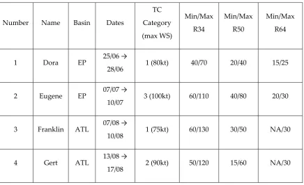
taken into account (Table 1). 117
Table 1. List and characteristics of the 16 hurricanes considered in this study. The minimum and 118
maximum radii at 34-kt, 50-kt, and 64-kts (R34, R50, and R64 respectively) are given in nautical miles 119
at the peak intensity. WS stands for wind speed. 120
Number Name Basin Dates
TC
Category
(max WS)
Min/Max
R34
Min/Max
R50
Min/Max
R64
1 Dora EP 25/06 →
28/06 1 (80kt) 40/70 20/40 15/25
2 Eugene EP 07/07 →
10/07 3 (100kt) 60/110 40/80 20/30
3 Franklin ATL 07/08 →
10/08 1 (75kt) 60/130 30/50 NA/30
4 Gert ATL 13/08 →
5 Harvey ATL 17/08 →
30/08 4 (115kt) 70/120 40/60 20/35
6 Hilary EP 24/08 →
30/08 2 (90kt) 60/90 30/50 15/20
7 Irma ATL 30/08 →
11/09 5 (160kt) 80/160 50/100 30/45
8 Irwin EP 23/07 →
01/08 1 (80kt) 30/60 10/30 NA/15
9 Jose ATL 05/09 →
22/09 4 (135kt) 50/120 30/50 20/30
10 Katia ATL 06/09 →
09/09 2 (90kt) 60/60 20/40 15/20
11 Kenneth EP 19/08 →
23/08 4 (115kt) 60/90 30/50 15/25
12 Lee ATL 16/09 →
30/09 3 (100kt) 60/80 40/50 25/30
13 Maria ATL 16/09 →
30/09 5 (150kt) 100/150 60/80 35/50
14 Max EP 13/09 →
15/09 1 (70kt) 30/40 20/20 10/10
15 Norma EP 14/09 →
19/09 1 (65kt) 70/80 30/50 NA/25
16 Otis EP 16/09 →
19/09 3 (100kt) 40/60 20/40 10/20
121
For each of these events, we considered the following data provided by the NHC (National 122
Hurricane Center) advisories: location of the cyclone center, minimum pressure, maximum wind 123
speed, radii of the 34-, 50-, and 64-knot winds in the four quadrants at every 6 hours. Most of these 124
data were calibrated using aircraft reconnaissance and are consequently expected to be reliable. 125
2.2. Remote sensing data 126
We also collected the full dataset distributed by the CYGNSS and ASCAT science team 127
The CYGNSS mission [31] consists of a eight satellites-constellation in low-inclination circular 129
orbit that receive direct and reflected GPS L1 (1.575 Ghz) signals to infer surface wind speeds and 130
sea roughness, even for intense rainfalls typically observed during hurricanes. It allows for a good 131
spatial and temporal coverage, with mean and median revisit times over the tropics of 7.2h and 2.8h 132
respectively [32]. The 25km- resolution data considered here (v2.0) have been validated and 133
calibrated using cyclones of the 2017 season, including most of the events considered in this study 134
(Table 1). For the time being, the overall root mean square (RMS) error in the CYGNSS retrievals is 135
about 1.4m/s and 17% for wind speeds lower and larger than 20 m/s respectively [40]. According to 136
the CYGNSS team (personal communication), the bias explains approximately half of the high wind 137
RMS (about 8.5%), the other half being random scatter. Generally speaking, we can thus expect 138
maximum biases of a few meters per second, even for high wind speeds. 139
140
We tested here several Level 2-wind speed products: 141
142
• The "wind speed" (ws) product is derived from the best fit to both the normalized bistatic radar 143
cross-section (NBRCS) and leading edge slope (LES) of the integrated delay waveform given by 144
the delay-Doppler maps (DDM [41]), using a fully developed seas geophysical model function 145
(GMF); 146
• The "yslf_les_wind_speed" (les) wind product is derived from only the LES of the DDM, using a 147
young seas / limited-fetch GMF; 148
• The "yslf_nbrcs_wind_speed" (nbrc) product is derived from only the NBRCS, using the young 149
seas / limited-fetch GMF. 150
151
ASCAT [22,42] consists of C-band scatterometers mounted on the satellites MetOp-A and 152
MetOp-B, that were launched in 2006 and 2012 respectively. The emitting antennas transmit pulses 153
at 5.255 GHz and extend on either side of the instrument, which results in a double 500km-wide 154
swath of observations. These scatterometers are found to give reliable estimations of wind speeds up 155
to at least 34-kt. However, they lose sensitivity in extreme conditions and are often plagued by rain 156
contamination. We use here the 25km-resolution coastal product, which give more wind data close 157
to the coast [43]. 158
2.3. Parametric wind models 159
For a given cyclone and parametric gradient wind profile, we estimated the surface wind speed 160
associated to each CYGNSS and ASCAT data point according to the following main steps: 161
162
1- From the NHC advisories, we estimated the surface background wind relative to the cyclone 163
translation velocity at the time of acquisition of the considered CYGNSS/ASCAT data point. 164
Following the approach of Lin and Chavas [17], we assumed that this wind is decelerated by a factor 165
α=0.56 and rotated counter-clockwise by an angle β=19.2° from the free tropospheric wind. 166
167
2-We removed the translational portion of the wind speed from the maximum observed wind 168
velocity and the 34-, 50-, and 64kt winds. 169
170
3-We converted surface velocities to velocities on top of the atmospheric boundary layer by 171
applying an empirical surface wind reduction factor SWRF [38]. In the following sections, we 172
specified SWRF=0.9. Other values were tested, but for the sake of simplicity results are not presented 173
here (they add very little to the conclusions of this paper). 174
175
4-We estimated the maximum wind radii for the four quadrants, using the chosen parametric 176
gradient wind profile, and the available wind radii information. For each quadrant, up to three radii 177
of maximum wind are thus obtained: one from the 64-kt wind radius (Rm64), another from the 50-kt
178
wind radius (Rm50), and a last one from the 34-kt wind radius (Rm34).
180
5-Depending on the available wind radii information considered, we computed Rm64, Rm34 or all
181
the radii of maximum winds (Rm64, Rm50, and Rm34) for the data point azimuth, using a spline
182
interpolation. 183
184
6-We computed the wind speed values at the CYGNSS/ASCAT data point obtained using the 185
chosen parametric gradient wind profile and the radii of maximum winds considered (Rm64, Rm34, or
186
all three of them). 187
7-We assessed the wind speed at the CYGNSS/ASCAT data point, using a weighted average of 188
the wind speeds obtained in the previous step. We followed the procedure proposed by Hu et al. 189
[44], which ensures that all the wind radii information is satisfied. 190
191
8-We obtained the surface wind speed by multiplying the result by SWRF. 192
193
9-The wind speed obtained in the previous step was combined with the surface background 194
wind computed in step 1 to get the final parametric wind speed at the CYGNSS/ASCAT data point 195
considered. 196
197
This procedure is repeated for all the storms, gradient wind profiles, and CYGNSS/ASCAT 198
Level 2-data points within a distance of 200km from the cyclone center. The parametric models 199
considered here are given in Table 2. 200
201
Table 2. Parametric wind models considered in this study. For all of them, an empirical surface wind 202
reduction factor [38] SWRF=0.9 was prescribed. Comparisons are only made for data within a 203
distance of 200km from the cyclone center. The translation vector is reduced by a factor α=0.56 and 204
rotated counter-clockwise by an angle β=19.2°, according to the findings of Lin and Chavas [17]. 205
Here, Vm and Rm are the maximum wind speed and the radius of maximum winds. r refers to the
206
distance to the TC center, and f to the coriolis coefficient. 207
Name Main reference Formula
E11 Emanuel and
Rotunno [36] ( ) =
2 ( 0.5 )
− 2
E04 Emanuel [45]
( ) =
−
(1 )( )
( )
(1 2 )
1 2
.
with b=0.25, m=1.6, n=0.9, R0=420km
J92 Jelesnianski et al [46] ( ) =2
H80 Holland [33] ( ) = ∆ −
with = ∆ , = 1.15, = exp (1)
H80c
Holland [33]
with cyclostrophic
approximation
( ) = ∆ −
with = ∆ , = 1.15, = exp (1)
M16 Murty et al. [37] ( ) = with = 3 5⁄
W06 Willoughby et al. [39]
For 0 ≤ ≤ : ( ) = with = 0.79
For ≥ : ( ) = − with = 243
208
3. Comparison of CYGNSS and ASCAT data 209
210
To get a preliminary idea of the usefulness of CYGNSS and ASCAT data as proxy for surface 211
wind speeds, we computed the biases between these data and the mean (i.e. averaged over all 212
empirical models) parametric winds for different cyclone categories and distances to the center 213
(Figure 1). Computations were performed only when more than 30 data points were available for a 214
given intensity/distance class. In practice, the comparison was possible for almost all cases, as 215
hundreds or even thousands of space-borne observations were available for each class. Parametric 216
models have been constrained by all the information provided by the NHC in the advisories, to 217
ensure that they give the best approximation possible to real winds. In classes for which the biases 218
are large, remote sensing data are not consistent with the mean parametric winds. We choose not to 219
investigate further these data in the following sections, even if there is no evidence that the error is 220
due to remote sensing rather than parametric models. On the contrary, small biases (in absolute 221
terms) suggest that remote sensing data and parametric winds are consistent, so that they both give 222
satisfactory results a priori. In the following, we will make the assumption that these 223
CYGNSS/ASCAT data are indeed good proxies, and check whether or not this hypothesis leads to 224
consistent results. 225
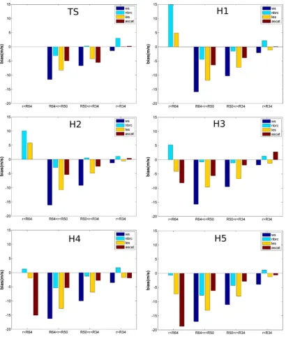
229
Figure 1. Bias between the remote sensing data and the parametric winds averaged over all 230
empirical models (negative/positive values indicate that remote sensing data are 231
negatively/positively biased compared to the mean parametric winds) . Different categories of 232
distance to the cyclone center (r) and cyclone intensities are considered. TS stands for tropical 233
storms, H1, H2, H3, H4, and H5 to the cyclone category (1, 2, 3, 4, and 5 respectively). R34, 234
R50, and R64 are the radii for the 34-kt, 50-kt, and 64-kt winds. ws, nbrc, and les are three 235
different CYGNSS products (see section 2). 236
237
Regarding ASCAT data, Figure 1 shows that the bias is low (less than about 2-3m/s in absolute 238
value) for radius larger than R34, but becomes increasingly negative with cyclone category and 239
decreasing distance to the cyclone center, up to almost -20m/s. These results suggest that ASCAT 240
data are a good proxy for wind speeds lower than 34-kt, but that they underestimate extreme winds. 241
This conclusion is consistent with previous published papers [47]. 242
The "wind speed" (ws) product is found to give systematically more negative biases than 243
ASCAT, and thus probably often underestimates the velocities (Figure 1). However, the absolute 244
might still be a good proxy for moderate and (potentially even more) low wind speeds. As this 246
product was developed for fully developed seas, these results were also expected. 247
Wind speeds derived from only the LES of the DDM ("les" in Figure 1) display, again, negative 248
biases for r>R64. However, those remain smaller in absolute value compared to "ws", which makes 249
sense since this product has been derived using a young seas / limited-fetch GMF that is expected to 250
be more suitable for our test cases. Considering the potential errors on parametric models, it could 251
be a proxy as good as ASCAT for radius larger than R34. Above all, this product shows significantly 252
reduced biases for r<R64. This suggests that it yields better estimates of surface wind speeds than 253
ASCAT close to the eyewall. 254
The wind speeds derived from only the NBRCS ("nbrc" in Figure 1) outperform the other 255
products in most cases for radius lower than R34, with bias generally lower than 5m/s in absolute 256
value. The main exception is the wind for radius lower than R64 for minor cyclones (category 1 or 2), 257
where the bias reaches 10 to 15m/s. One plausible explanation is that the resolution of CYGNSS 258
(25km) is too low to capture the surface wind speeds in these area, especially for weak cyclones 259
where the 64kt radii are very close to the eyewall, i.e. to places where wind speeds vary quickly as a 260
function of distance to the center. This problem is presumably less severe for major cyclones 261
(category 3 or more) because of a larger extent of hurricane-force winds (Table 1). 262
263
Based on all these findings, we will hypothesize in the following section that the ASCAT and 264
CYGNSS/NBRC products are the best surface wind speeds proxy for r> R34 and r<R34 respectively. 265
However, we will not consider radii lower than R64 for weak (category 1-2) cyclones, as Figure 1 266
also suggest that none of the space-borne products tested here is reliable in these conditions. 267
268
We will check in sections 4 and 5 whether these preliminary results and assumptions give 269
results consistent with previous work and in-situ data, to confirm or invalidate them a posteriori. 270
4. Performance of parametric wind models 271
Using the assumption made in the previous section, we computed the bias of the various 272
parametric models as a function of storm intensity, distance to the cyclone center, and calibration 273
method (using only radii at 34kt, only radii at 64kt, and all radii information for the left, middle and 274
right panels respectively in Figure 2). The color bar shows the absolute value of bias. Blue colors 275
correspond to small biases (in absolute value), and thus suggest that the parametric model should 276
work well for the intensity/distance class considered. Conversely, red colors indicate that the model 277
is expected to perform poorly. The aim is to see whether the assumption on which this figure is 278
based ("ASCAT and CYGNSS/NBRC are good wind speeds proxy for r> R34 and r<R34 279
respectively") gives consistent results or not. 280
Figure 2. Diagrams displaying the bias between various parametric models and the surface 283
wind speeds estimated by CYGNSS/ASCAT data for all the events considered here, as a function of 284
storm intensity and distance to the cyclone center (x- and y-axis respectively for each diagram), as 285
well as calibration method (using only radii at 34kt, only radii at 64kt, and all radii information for 286
the left, middle and right panels respectively). The color bar (the same for all diagrams) shows the 287
absolute value bias. The values are displayed for each category/distance cell. The black contours 288
indicate the category/distance classes for which we consider E11 and H80 models in section 5 (model 289
E11H80). 290
First of all, it appears that the bias is significantly reduced in almost all cases for r<R64 and r>R34 291
when constraining the parametric models by R64 and R34 respectively. This suggests that not only 292
the "mean" parametric wind values computed in section 3 are consistent with the CYGNSS/ASCAT 293
data for these classes, but also most of the parametric models taken individually, as long as they are 294
constrained by the 64-kt and 34-kt wind radii given by the NHC. This finding gives additional credit 295
to the assumption we made in section 3. It may, however, be observed that biases are not always so 296
much reduced (and can even be increased) when constraining the parametric models by R50 for very 297
intense (category >3) cyclones. This issue appears also in Figure 1, where strangely the absolute bias 298
of CYGNSS is larger for R64<r< R50 than for r<R64. There could be several explanations to this fact: 299
an issue with the calibration of CYGNSS data for these conditions of course, but also a problem with 300
the parametric models for extreme events in the "transition zone" (the area between the inner 301
core/outer region). The latter cannot be dismissed, as most parametric models were built by focusing 302
mainly on the inner and/or outer regions (e.g. [39]), whereas much less attention was paid to the 303
transition zone between extreme and moderate winds. We will return to this point later on. 304
The results are also found to be consistent with most of the previous works. For instance: 305
• The inner region solution of Emanuel and Rotunno [36], E11, generally gives the smaller bias 306
(hence the best results) close to the storm center (typically, for r<R50), especially for intense and 307
well defined cyclones. It is also found to underestimate significantly the wind speeds far from 308
the center as found in Lin and Chavas [17], even when prescribing the radii at 34-kt. E04 309
performs much better for the outer region, but poorly near the center. E11 and E04 can thus be 310
merged to develop a complete TC radial wind structure as proposed by Chavas et al. [48]; 311
• When solely constrained by radii close to the cyclone center (here R64), the Holland profile 312
(H80) tends to underestimate the winds in the outer region, as noted by Willoughby and Rahn 313
[34]. It can also lead to broad wind maximum, and thus wind overestimations at several dozens 314
of kilometers from the center for extreme cyclones (for R64<r<R50 for example), as can be seen 315
in the right and left panels notably. These findings, which are in accordance with the results of 316
Willoughby and Rahn [34], confirm that the issue we identified earlier with the 50-kt wind radii 317
could be partly due to flaws in parametric models such as H80 in the "transition zone". 318
• J92 tends to overestimate the wind speeds by a few m/s, as suggested by Lin and Chavas [17]; 319
• The results are generally much better when considering a family of profiles with two 320
characteristic lengths, as proposed by Willoughby et al [39]. For example, as stated above, the 321
performance of the Holland model H80 is significantly increased when both radii at 34-kt and 322
64-kt are prescribed; 323
• Models such as W06 or M16 (which decay exponentially or as a power-law outside the eye) 324
perform well in the outer region when the 34-kt radii are prescribed properly, which is 325
consistent with the findings of Willoughby et al. [39] and Murty et al. [37]. 326
The consistency of these results increases the confidence in our assumption that the ASCAT and 327
CYGNSS/NBRC products are relatively good proxies for surface wind speeds, for r>R34 and r<R34 328
respectively (with the exception of the inner region for weak cyclones). To further build the 329
confidence in this hypothesis, we also performed numerical hindcasts of hurricane Maria (2017), and 330
investigate the potential of results such as those presented in Figure 2 to choose one parametric 332
model rather than another, depending on the case study. 333
5. Comparison with in-situ data 334
Hurricane Maria was the deadliest storm of the 2017 Atlantic season. Recorded as a category 5 335
event, it caused catastrophic damages in Dominica and Puerto Rico, as well as widespread flooding 336
and crop destructions in Guadeloupe. We tested here the ability of several parametric models to 337
properly represent the wind pattern evolution during Maria by comparing the significant wave 338
heights observed at buoys in the Lesser Antilles with those computed using a wave-current coupled 339
model forced by a sub-set of the various parametric winds considered in the previous section. The 340
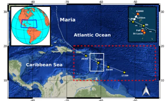
model is based on the code SCHISM-WWM [49]. The computational domain is represented in Figure 341
3. Resolution spans from 10km far from the region of interest (where the bathymetry is derived from 342
GEBCO), up to about 100m in Guadeloupe and Martinique where we have the best bathymetric data 343
(ship-based soundings from the SHOM, the French Naval Hydrographic and Oceanographic 344
Department). The model is forced by: 345
• astronomic tidal potential over the whole domain (12 constituents); 346
• 26 tidal harmonic constituents at the open boundaries, provided by the global FES2012 model 347
[50] ; 348
• parametric pressure fields [33]; 349
• parametric winds blended with CFSR (Climate Forecast System Reanalysis [51]) wind data. The 350
parametric winds are prescribed for radii less than R34 , whereas CFSR data are imposed for r > 351
1.5 R34. In between, a smooth transition is ensured using a weighing coefficient varying with 352
the radius r. 353
354
355
Figure 3. Study area. The computational domain is depicted with the dashed red contour. The 356
dashed white line represents the track of hurricane Maria. The location of the buoys used for 357
comparison is given in the upper-right corner box. 358
359
We considered here five parametric models: 360
• E11 and H80, constrained using the 64-kt wind radii only (E11(R64) and H80(R64) in Figure 4); 361
• E11 and H80, constrained using all the wind radii information (E11(All) and H80(All) in Figure 362
4); 363
• E11H80, for which we chose to blend the wind speeds inferred from E11 for the inner core area 364
with those given by H80 for the outer region (see the black contours in Figure 2) 365
366
E11H80 was chosen to test whether results such as those presented in Figure 2 could be of benefit to 367
build a better parametric model for the cyclone considered, using a combination of models that is 368
is just an example. In no way we consider this model as the best option. E11 combined with W06 or 370
E04 could be also tested for instance. 371
372
The reader is referred to Krien et al [9] for greater details about the model and the numerical 373
strategy. Here, we compared the significant wave heights (Hs) computed by the model with the Hs 374
recorded by three buoys located in the Lesser Antilles (Figure 3): Fort de France (FdF) and Sainte 375
Lucie, owned by Meteo France, as well as 42060, maintained by the National Data Buoy Center 376
(NDBC). The latter went adrift during the peak of Maria, hence the decrease of Hs was unfortunately 377
not captured. 378
379
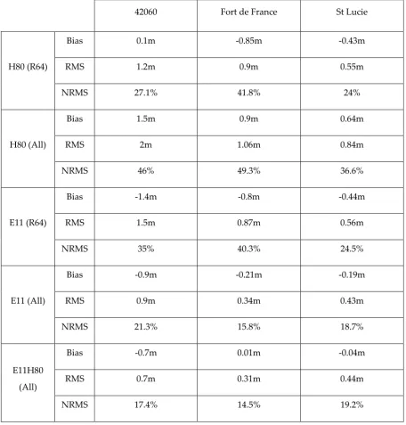
Table 3. Bias, root mean square error (RMS) and normalized RMS (NRMS) obtained when 380
comparing numerical simulations with in-situ significant wave heights. 381
42060 Fort de France St Lucie
H80 (R64)
Bias 0.1m -0.85m -0.43m
RMS 1.2m 0.9m 0.55m
NRMS 27.1% 41.8% 24%
H80 (All)
Bias 1.5m 0.9m 0.64m
RMS 2m 1.06m 0.84m
NRMS 46% 49.3% 36.6%
E11 (R64)
Bias -1.4m -0.8m -0.44m
RMS 1.5m 0.87m 0.56m
NRMS 35% 40.3% 24.5%
E11 (All)
Bias -0.9m -0.21m -0.19m
RMS 0.9m 0.34m 0.43m
NRMS 21.3% 15.8% 18.7%
E11H80
(All)
Bias -0.7m 0.01m -0.04m
RMS 0.7m 0.31m 0.44m
NRMS 17.4% 14.5% 19.2%
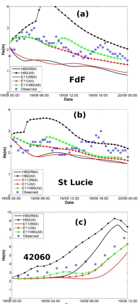
Results (Table3, Figure 4) show that: 382
• H80 and E11 constrained only by the 64-kt wind radii (R64) give the worst results, with Hs 383
• Trying to improve these models by constraining all the 34-kt, 50-kt, and 64-kt wind radii (All) 385
results in much better performances for E11, with reduced bias and NRMS (15 to 22% 386
approximately). This suggests that E11 satisfactorily represents the TC structure, at least as long 387
as the hurricane (here in category 4-5) remains relatively close to the buoys. It tends to 388
underestimate Hs (in Sainte Lucie for example) when the storm moves further away. 389
• On the contrary, the H80 model strongly overestimates Hs when Maria is the closest to the 390
storm, at a distance of about 120-200km (which corresponds roughly to the radii at 50-kt). This 391
is also consistent with the results of Figure 2, and confirms, again, that the relatively significant 392
biases obtained in Figure 1 for extreme cyclones and R64<r<R50 might be partly explained by 393
flaws in parametric models such as H80 rather than errors in CYGNSS wind speeds. The 394
prediction is better when Maria moves further away, which was also expected. 395
• The best results are obtained here for the model E11H80. The bias is found to be considerably 396
reduced compared to E11constrained with all wind radii. 397
398
These results are all consistent with those presented in Figure 2 (keeping in mind that Maria is 399
here a category 4-5 hurricane, and that it passes relatively close to the buoys, see Figure 3). Hence 400
they also support our assumption that the ASCAT and CYGNSS/NBRC products are relatively good 401
proxies for surface wind speeds, for r>R34 and r<R34 respectively (with the exception of the inner 402
region for weak cyclones). 403
407
Figure 4- Significant wave height time series for different parametric models. "R64" denotes a 408
model constrained only by the 64-kt wind radii. "ALL" indicates a model constrained with all 409
the available information (34-kt, 50-kt, and 64-kt wind radii). E11H80 corresponds to a blend of 410
the model E11 (for the inner core region) and H80 (for the outer region). Results for 411
Fort-de-France, Sainte-Lucie, and the 42060 station are displayed in (a), (b), and (c) respectively. 412
6. Conclusions 414
Taking advantage of an extremely active 2017 hurricane season in the tropical Atlantic Ocean and the 415
Eastern Pacific, we investigated the potential of using recent satellite remote sensing data such as CYGNSS and 416
ASCAT to identify the advantages and drawbacks of several parametric wind models used for storm surge 417
hazard assessment or prediction of cyclonic waves. 418
Under the assumption that ASCAT and CYGNSS/NBRC products can be considered as good proxies for surface 419
wind speeds for the outer and inner regions respectively (with an exception for the core of weak cyclones), we 420
were able to confirm the findings of a number of previous studies (e.g. Willoughby et al. [39], Lin and Chavas 421
[17] or Chavas et al. [48]). Using a wave-current coupled numerical model, we also showed that remote sensing 422
data such as CYGNSS/ASCAT are probably sufficiently accurate to be used to better select a suitable parametric 423
model, depending on the case study considered. The choice will depend on several criteria such as cyclone 424
intensity and/or availability of wind radii information. Indeed, our results suggest that none of the traditional 425
empirical approaches can be considered as the best option in all cases. 426
We strongly insist on the fact that our aim here is not to encourage using or discarding a specific parametric 427
model, and even less to propose a new one. First, because we did not test all the published models. Second, 428
because each author uses a specific combination of parameters and approach to mimic the wind field, so that it 429
would be presumptuous to draw definitive conclusions. Besides, there are still errors on remote sensing data, so 430
that differences of 2-3m/s in terms of bias are probably not really significant. 431
The main finding of this paper is thus the following: satellite remote sensing is now mature enough to provide 432
relevant information about the performance of parametric cyclonic wind models, even if further work is 433
needed, especially to access to the full structure of TCs close to the eyewall. We focused here mainly on the 434
CYGNSS mission, but there is little doubt that other type of data can also be valuable. Remote sensing has now 435
become a powerful tool that should be used to validate or improve existing parametric approaches, in order to 436
conduct better wind, waves, and surge analysis for TCs. 437
It is noteworthy to conclude by mentioning that even with the improved model tested here for Maria (see 438
section 5), the NRMS remains relatively high (15-20%). Indeed, the temporal resolution (6-hours) is not 439
sufficient to allow parametric models to reproduce the short-term variations of track, translation speed, or wind 440
asymmetry. This stresses the need for higher temporal sampling of data (location of the cyclone center, 441
maximum wind speed, wind radii, etc), and greater efforts to improve the efficiency of numerical atmospheric 442
models. 443
Acknowledgments: This study was founded by the ERDF/C3AF project as well as the IRD. Our warm thanks to 444
the CYGNSS and ASCAT science team members for their work. ASCAT and CYGNSS data were provided by 445
the KNMI and PODAAC data center respectively. Data at Fort-de-France and Sainte-Lucie were made available 446
by the CEREMA (CANDHIS database).The significant wave heights at station 42060 were provided by NDBC. 447
Author Contributions: Yann Krien conceived the idea and wrote most of the paper; Gaël Arnaud, Raphaël 448
Cécé and Jamal Khan contributed to the development of the analysis tools; Gaël Arnaud, Ali Bel Madani and 449
A.K.M.S. Islam arranged the figures and corrected a number of errors in the first version of the manuscript. 450
Didier Bernard, Philippe Palany and Narcisse Zahibo prepared the project C3AF which funded about 66% of 451
the work presented here. Fabien Durand, Laurent Testut and A.K.M.S. Islam played a major role for obtaining 452
the IRD grant (about one third of total fundings). The manuscript also greatly benefited from their 453
proofreading and suggestions. 454
Conflicts of Interest: The authors declare no conflict of interest. 455
References 456
1. Vickery, P. J., Masters, F.J., Powell, M.D., Wadhera, D. Hurricane hazard modeling: The past, present, and 457
future, J. Wind Eng. Ind. Aerodyn. 2009, 97, 392–405, doi:10.1016/j.jweia.2009.05.005. 458
2. Lin, N., Smith, J.A., Villarini, G., Marchok, T.P., Baeck, M.L. Modeling extreme rainfall, winds, and surge 459
from Hurricane Isabel (2003), Weather Forecast. 2010, 25, 1342–1361, doi:10.1175/2010WAF2222349.1. 460
3. Hsiao, L. F., Chen, D.S., Kuo, Y.H., Guo, Y.R., Yeh, T.C., Hong, J.S., Fong, C.T., Lee, C.S. Application of 461
WRF 3DVAR to operational typhoon prediction in Taiwan: Impact of outer loop and partial cycling 462
approaches. Wea. Forecasting2012, 27, 1249–1263, doi:10.1175/WAF-D-11-00131.1. 463
4. Powers, J., Klemp, J., Skamarock, W., Davis, C., Dudhia, J., Gill, D., Coen, J., Gochis, D., Ahmadov, R., 464
Schwartz, C., Romine, G., Liu, Z., Snyder, C., Chen, F., Barlage, M., Yu, W., Duda, M. The weather research 466
and forecasting (WRF) model: overview, system efforts, and future directions. Bull. Am. Meteorol. Soc.2017, 467
http://dx.doi.org/10.1175/BAMS-D-15-00308.1 468
5. Lakshmi, D., Murty, P.L.N., Bhaskaran, P.K., Sahoo, B., Srinivasa Kumar, T., Shenoi, S.S.C., Srikanth, A.S. 469
Performance of WRF-ARW winds on computed storm surge using hydrodynamic model for Phailin and 470
Hudhud cyclones. Ocean. Eng.2017, 131, 135–148. 471
6. Mattocks C., Forbes C. A real-time, event-triggered storm surge forecasting system for the state of North 472
Carolina. Ocean. Model.2008, 25:95–119. 473
7. Lin, N., Emanuel, K.A. Grey swan tropical cyclones. Nat. Climate Change 2016, 6, 106–111, 474
doi:10.1038/nclimate2777. 475
8. Orton, P. M., Hall, T.M., Talke, S.A., Blumberg, A.F., Georgas, N., Vinogradov, S. A validated 476
tropical-extratropical flood hazard assessment for New York harbor. J. Geophys. Res. Oceans2016, 121, 477
8904–8929, https://doi.org/10.1002/2016JC011679. 478
9. Krien, Y., Testut, L., Durand, F., Mayet, C., Islam A.K.M.S., Tazkia, A.R., Becker, M., Calmant, S., Papa, F., 479
Ballu, V., Shum, C.K., Khan, Z.H. Towards improved storm surge models in the northern Bay of Bengal. 480
Continental Shelf Research2017, 135, 58-73. 481
10. Shao, Z., Liang, B., Li, H., Wu, G., Wu, Z. Blended wind fields for wave modeling of tropical cyclones in 482
the South China Sea and East China Sea. Applied Ocean Research2018, 71, 20-33. 483
11. Feng, X., Li, M., Yin, B., Yang, D., Yang, H. Study of storm surge trends in typhoon-prone coastal areas 484
based on observations and surge-wave coupled simulations. Int. J. Appl. Earth Obs. Geoinf. 2018, 485
https://doi.org/10.1016/j.jag.2018.01.006. 486
12. Tan, C., Fang, W. Mapping the Wind Hazard of Global Tropical Cyclones with Parametric Wind Field 487
Models by Considering the Effect of Local Factors. Int. J. Disaster Risk Sci. 2018, 488
https://doi.org/10.1007/s13753-018-0161-1. 489
13. Niedoroda, A. W., Resio, D. T., Toro, G. R., Divoky, D., Das, H. S., and Reed, C. W. Analysis of the coastal 490
Mississippi storm surge hazard, Ocean Eng.2010, 37, 82–90. 491
14. Haigh, I. D., MacPherson, L. R., Mason, M. S.,Wijeratne, E. M. S., Pattiaratchi, C. B., Crompton, R. P., and 492
George, S. Estimating present day extreme water level exceedance probabilities around the coastline of 493
Australia: tropical cyclone-induced storm surges, Clim. Dynam.2014, 42, 139–157. 494
15. Krien, Y., Dudon, B., Roger, J., Zahibo, N. Probabilistic hurricane-induced storm surge hazard assessment 495
in Guadeloupe, Lesser Antilles. Nat. Haz. Earth Syst. Sci.2015, 15, 1711-1720. 496
16. Krien, Y., Dudon, B., Roger, J., Arnaud, G., Zahibo, N. Assessing storm surge hazard and impact of sea 497
level rise in Lesser Antilles-Case study of Martinique. Nat. Haz. Earth Syst. Sci.2017, 17, 1559-1571. 498
17. Lin, N., Chavas, D. On hurricane parametric wind and applications in storm surge modeling. J. Geophys. 499
Res.2012, 117, D09120. http://dx.doi.org/10.1029/2011JD017126. 500
18. Olfateh, M., Callaghan, D.P., Nielsen, P., Baldock, T.E. Tropical cyclone wind field 501
asymmetry—development and evaluation of a new parametric model, J. Geophys. Res. Oceans2017, 122, 502
458–469. 503
19. Knaff, J.A., S.P. Longmore, R.T. DeMaria, Molenar, D.A. Improved Tropical-Cyclone Flight-Level Wind 504
Estimates Using Routine Infrared Satellite Reconnaissance. J. Appl. Meteor. Climatol. 2015, 54, 463-478. 505
20. Dolling, K., E. Ritchie, Tyo, J. The Use of the Deviation Angle Variance Technique on Geostationary 506
Satellite Imagery to Estimate Tropical Cyclone Size Parameters. Wea. Forecasting2016, 31, 1625–1642, doi: 507
10.1175/WAF-D-16-0056.1. 508
21. Mueller, K. J., DeMaria, M., Knaff, J.A., Kossin, J.P., Vonder Haar, T.H. Objective estimation of tropical 509
cyclone wind structure from infrared satellite data. Wea. Forecasting 2006, 21, 990–1005, 510
doi:10.1175/WAF955.1. 511
22. Figa-Saldana, J., Wilson, J.J.W., Attema, E., Gelsthorpe, R., Drinkwater, M.R., Stoffelen, A. The advanced 512
scatterometer (ASCAT) on the meteorological operational (MetOp) platform: A follow on for European 513
wind scatterometers. Canadian Journal of Remote Sensing2002, 28, 404-412. 514
23. Madsen, N. M., Long, D.G. Calibration and Validation of the RapidScat Scatterometer Using Tropical 515
Rainforests. IEEE Trans. Geosci. Remote Sens.2016, 54, 2846-2854. 516
24. Meissner, T., Wentz, F.J. Wind vector retrievals under rain with passive satellite microwave radiometers, 517
25. El-Nimri, S. F., Lindwood Jones, W., Uhlhorn, E., Ruf, C., Johnson, J., Black, P. An improved C-band ocean 519
surface emissivity model at hurricane-force wind speeds over a wide range of Earth incidence angles, 520
IEEE Geosci. Remote Sens. Lett. 2010, 7, 641–645, doi:10.1109/LGRS.2010.2043814. 521
26. Reul N., Tenerelli J., Chapron B., Vandemark D., Quilfen Y., Kerr, Y. SMOS satellite L-band radiometer: A 522
new capability for ocean surface remote sensing in hurricanes. Journal of Geophysical Research2012, vol. 117, 523
C02006, doi: 10.1029/2011JC007474. 524
27. Reul N., Chapron B., Zabolotskikh E., Donion C., Mouche A.A., Tenerelli J., Collard F., Piolle J.F., Fore A., 525
Yueh S., Cotton J., Francis P., Quilfen Y., Kudryavtsev V. A new generation of tropical cyclone size 526
measurements from space. Bull. Am. Meteorol. Soc. 2017, 98: 2367–2385, 527
https://doi.org/10.1175/BAMS-D15-00291.1. 528
28. Zabolotskikh E., Mitnik L. M., Reul N., Chapron B. New Possibilities for Geophysical Parameter Retrievals 529
Opened by GCOM-W1 AMSR2. IEEE Journal of Selected Topics in Applied Earth Observations and Remote 530
Sensing2015, PP(99), 1-14. Publisher's official version : http://dx.doi.org/10.1109/JSTARS.2015.241651. 531
29. Fore, A. G., Yueh, S.H., Tang, W., Stiles, B., Hayashi, A.K. Combined Active/Passive Retrievals of Ocean 532
Vector Wind and Sea Surface Salinity With SMAP. IEEE Trans. Geosci. Remote Sens.2016, 54(12), 7396-7404. 533
30. Foti, G., Gommenginger, C., Jales, P., Unwin, M., Shaw, A., Robertson, C., Rosell, J. Spaceborne GNSS 534
reflectometry for ocean winds: First results from the UK TechDemoSat-1 mission. Geophys. Res.Lett. 2015, 535
vol. 42, no. 13, pp. 5435–5441. http://dx.doi.org/10.1002/2015GL064204 536
31. Ruf, C., and Coauthors. New Ocean Winds Satellite Mission to Probe Hurricanes and Tropical Convection. 537
Bull. Amer. Meteor. Soc.2016, 97, 385-395, doi:10.1175/BAMS-D-14-00218.1. 538
32. Morris, M., Ruf, C. Determining Tropical Cyclone Surface Wind Speed Structure and Intensity with the 539
CYGNSS Satellite Constellation. J. Appl. Meteor. Climatol. 2017, doi:10.1175/JAMC-D-16-0375.1 540
33. Holland, G. An Analytic Model of the Wind and Pressure Profiles in Hurricanes. Monthly Weather Review 541
1980, 108:1212–1218. 542
34. Willoughby, H.E., Rahn, M.E. Parametric representation of the primary hurricane vortex. Part I: 543
Observations and evaluation of the Holland (1980) model. Mon. Wea. Rev. 2004, 132, 3033–3048. 544
35. Jelesnianski, C.P., Taylor, A.D. A preliminary view of storm surges before and after storm modifications. 545
NOAA Technical Memorandum. ERL WMPO-3, National Oceanic and Atmospheric Administration, U.S. 546
Department of Commerce1973, pp.33. 547
36. Emanuel, K., Rotunno, R. Self-stratification of tropical cyclone outflow, Part I: Implications for storm 548
structure, J. Atmos. Sci. 2011, 68, 2236–2249. 549
37. Murty, P.L.N., Bhaskaran, P.K., Gayathri, R., Sahoo, B., Srinivasa Kumar, T., SubbaReddy, B. Numerical 550
study of coastal hydrodynamics using a coupled model for Hudhud cyclone in the Bay of Bengal, 551
Estuarine, Coastal and Shelf Science2016, doi: 10.1016/j.ecss.2016.10.013. 552
38. Powell, M. D., Vickery, P.J., Reinhold, T.A. Reduced drag coefficient for high wind speeds in tropical 553
cyclones, Nature2003, 422(6929), 279–283, doi:10.1038/nature01481. 554
39. Willoughby, H. E., Rahn, M. E., Darling, R. W. R. Parametric representation of the primary hurricane 555
vortex. Part II: A new family of sectionally continuous profiles. Mon. Weath. Rev.2006, 134, 1102–1120. 556
40. Ruf, C. S., Gleason, S., McKague, D.S. Assessment of CYGNSS Wind Speed Retrieval Uncertainty. IEEE J. 557
Sel. Topics Appl. Earth Obs. Remote Sens. 2018. DOI:10.1109/JSTARS.2018.2825948. 558
41. Saïd, F., Katzberg, S.J., Soisuvarn, S. Retrieving Hurricane Maximum Winds Using Simulated CYGNSS 559
Power-Versus-Delay Waveforms. IEEE Journal of Selected Topics in Applied Earth Observations and Remote 560
Sensing2017. DOI:10.1109/JSTARS.2017.2695878 561
42. ASCAT Wind Product User Manual, KNMI, De Bit, The Netherlands, 2013. [Online]. Available: 562
http://projects.knmi.nl/ scatterometer/publications/pdf/ASCAT_Product_Manual.pdf 563
43. Verhoef, A., Portabella, M., and Stoffelen, A. High-resolution ASCAT scatterometer winds near the coast. 564
IEEE Trans. Geosci. Remote Sens. 2012, vol. 50, no. 7, pp. 2481–2487, doi:10.1109/TGRS.2016.2544835 565
44. Hu, K., Chen, Q., Kimball, S.K. Consistency in hurricane surface wind forecasting : an improved 566
parametric model. Nat. Hazards2012, 61, 1029-1050. 567
45. Emanuel, K. Tropical cyclone energetics and structure, in Atmospheric Turbulence and Mesoscale 568
Meteorology, edited by E. Fedorovich, R. Rotunno, and B. Stevens 2004, pp. 165–192, Cambridge Univ. 569
Press, Cambridge, U. K., doi:10.1017/CBO9780511735035.010. 570
46. Jelesnianski, C. P., Chen, J., Shaffer, W.A. SLOSH: Sea, lake, and overland surges from hurricanes, NOAA Tech. 571
47. Brennan, M.J, Hennon, C.C., Knabb, R.D. The Operational Use of QuikSCAT Ocean Surface Vector Winds 573
at the National Hurricane Center. Weather and Forecasting2009, 24, 621-645. 574
48. Chavas, D. R., Lin, N., Emanuel, K. A model for the complete radial structure of the tropical cyclone wind 575
field. Part I: Comparison with observed structure. J. Atmos. Sci. 2015, 72, 3647–3662, 576
doi:https://doi.org/10.1175/JAS-D-15-0014.1 577
49. Zhang, Y., Ye, F., Stanev, E.V., Grashorn, S. Seamless cross-scale modeling with SCHISM. Ocean Modelling 578
2016, 102, 64–81. 579
50. Carrère, L., Lyar, F., Cancet, M., Guillot, A., Roblou, L. FES2012: A new global tidal model taking 580
advantage of nearly 20 years of altimetry. In: Paper presented at Proceedings of The Symposium 20 Years of 581
Progress in Radar Altimetry, 2012, Venice. 582
51. Saha, S., et al. NCEP Climate Forecast System Version 2 (CFSv2) Monthly Products. Research Data Archive at 583
the National Center for Atmospheric Research, Computational and Information Systems Laboratory, 2012, 584
![Table 2. Parametric wind models considered in this study. For all of them, an empirical surface wind reduction factor [38] SWRF=0.9 was prescribed](https://thumb-us.123doks.com/thumbv2/123dok_us/7929171.1316601/6.595.70.525.465.785/table-parametric-models-considered-empirical-surface-reduction-prescribed.webp)