Western University Western University
Scholarship@Western
Scholarship@Western
Electronic Thesis and Dissertation Repository
11-15-2013 12:00 AM
Hardware Acceleration Technologies in Computer Algebra:
Hardware Acceleration Technologies in Computer Algebra:
Challenges and Impact
Challenges and Impact
Sardar Anisul Haque
The University of Western Ontario Supervisor
Dr. Marc Moreno Maza
The University of Western Ontario Graduate Program in Computer Science
A thesis submitted in partial fulfillment of the requirements for the degree in Doctor of Philosophy
© Sardar Anisul Haque 2013
Follow this and additional works at: https://ir.lib.uwo.ca/etd
Part of the Numerical Analysis and Scientific Computing Commons, and the Other Computer Sciences Commons
Recommended Citation Recommended Citation
Haque, Sardar Anisul, "Hardware Acceleration Technologies in Computer Algebra: Challenges and Impact" (2013). Electronic Thesis and Dissertation Repository. 1803.
https://ir.lib.uwo.ca/etd/1803
This Dissertation/Thesis is brought to you for free and open access by Scholarship@Western. It has been accepted for inclusion in Electronic Thesis and Dissertation Repository by an authorized administrator of
Hardware Acceleration Technologies in Computer Algebra: Challenges and Impact
(Thesis format: Monograph)
by
Sardar Anisul Haque
Graduate Program in
Computer Science
A thesis submitted in partial fulfillment of the requirements for the degree of
Doctor of Philosophy
The School of Graduate and Postdoctoral Studies The University of Western Ontario
London, Ontario, Canada
c
Abstract
The objective of high performance computing (HPC) is to ensure that the compu-tational power of hardware resources is well utilized to solve a problem. Various techniques are usually employed to achieve this goal. Improvement of algorithm to reduce the number of arithmetic operations, modifications in accessing data or rear-rangement of data in order to reduce memory traffic, code optimization at all levels, designing parallel algorithms with smaller span or reduced overhead are some of the attractive areas that HPC researchers are working on.
In this thesis, we investigate HPC techniques for the implementation of basic routines in computer algebra targeting hardware acceleration technologies. We start with a sorting algorithm and its application to sparse matrix-vector multiplication for which we focus on work on cache complexity issues. Since basic routines in computer algebra often provide a lot of fine grain parallelism, we then turn our attention to many-core architectures on which we consider dense polynomial and matrix operations ranging from plain to fast arithmetic. Most of these operations are combined within a bivariate system solver running entirely on a graphics processing unit (GPU).
Acknowledgments
I would like to thank my thesis supervisor Dr. Marc Moreno Maza in the department of Computer Science at the University of Western Ontario. His helping hands toward the completion of this research work were always extended for me. He consistently helped me on the way of this thesis and guided me in the right direction whenever he thought I needed it. I am grateful to him for his excellent support to me in all the steps of successful completion of this research.
I want to thank Dr. Wei Pan of Intel Corporation for discussions around our CUDA implementation for condensation method in the finite field case. Many thanks to Dr. J¨urgen Gerhard of Maplesoft for his help during my internship. My sincere thanks to Dr. Shahadat Hossain in the Department of Computer Science at the University of Lethbridge for taking the time to share his thoughts on sparse matrices with me.
I want to thank Dr. Yuzhen Xie, Dr. Changbo Chen in the Department of Com-puter Science at the University of Western Ontario for providing me help and sharing their knowledge.
All my sincere thanks and appreciation go to all the members from our Ontario Research Center for Computer Algebra (ORCCA) lab, Computer Science Department for their invaluable teaching support as well as all kinds of other assistance.
Many thanks to the members of my committee Dr. ´Eric Schost, Dr. Michael Bauer, Dr. Kenneth A. McIsaac of the University of Western Ontario and Dr. Yuxiong He of Microsoft Research for their reading of this thesis and comments.
Finally, I would like to thank all of my friends and family members for their consistent encouragement and support.
Contents
Abstract ii
Acknowledgments iii
Table of Contents iv
List of Algorithms viii
List of Figures x
List of Tables xii
1 Introduction 1
2 Background 4
2.1 Random access machine (RAM) model . . . 4
2.2 The PRAM model . . . 5
2.2.1 Parallel time, efficiency and speedup factor . . . 7
2.2.2 Different types of PRAM models . . . 7
2.3 The ideal cache model . . . 8
2.4 The multi-core machine model . . . 10
2.5 The fork-join parallelism model . . . 12
2.5.1 The work law . . . 13
2.5.2 The span law . . . 13
2.5.3 Parallelism . . . 13
2.5.4 Performance bounds . . . 14
2.5.5 Work, span and parallelism of classical algorithms . . . 14
3 Many-core Machine Model 16
3.1 Introduction . . . 16
3.2 A many-core machine model . . . 18
3.2.1 Many-core machine characteristics . . . 19
3.2.2 Many-core machine programs . . . 21
3.2.3 Complexity measures for the many-core machine model . . . . 23
3.2.4 A Graham-Brent theorem with overhead . . . 24
3.2.5 Justification of the many-core machine model . . . 24
4 Cache-oblivious Counting Sort Algorithm 26 4.1 Introduction . . . 26
4.2 The classical counting sort algorithm . . . 27
4.3 Cache-oblivious counting sort algorithm . . . 28
4.4 Experiments . . . 34
4.5 Conclusion . . . 34
5 A New Integer Sorting Algorithm 36 5.1 Introduction . . . 36
5.2 Notations . . . 37
5.3 Cost of the comparand function for large integers . . . 38
5.4 A new sorting algorithm . . . 39
5.4.1 Creating Ak+1 fromAk . . . . 40
5.5 Complexity . . . 43
5.6 Conclusion . . . 44
6 Cache Friendly Sparse Matrix-vector Multiplication 45 6.1 Introduction . . . 45
6.2 Background . . . 46
6.2.1 Compressed row storage scheme (CRS) . . . 47
6.2.2 SpMxV with CRS scheme . . . 47
6.2.3 Compressed column storage scheme (CCS) . . . 47
6.2.4 Notations . . . 47
6.2.5 Binary reflected Gray code . . . 48
6.2.6 Sorting of binary reflected Gray codes . . . 48
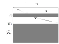
6.3 Proposed reordering method . . . 49
6.3.1 Initial column ordering . . . 51
6.3.3 Algorithm merge(A1, b, m) . . . . 54
6.3.4 Iterative column ordering . . . 54
6.4 Complexity . . . 56
6.4.1 Time complexity . . . 56
6.4.2 Memory complexity . . . 56
6.4.3 Cache complexity . . . 56
6.5 Experimental results . . . 59
6.6 Conclusion . . . 60
7 Implementation of Determinant by Condensation Method on GPU 63 7.1 Introduction . . . 63
7.2 The condensation method . . . 64
7.2.1 The formula of Salem and Said . . . 65
7.2.2 The algebraic complexity of the condensation method . . . 65
7.2.3 The cache complexity of condensation method . . . 66
7.3 GPU implementation: the finite field case . . . 67
7.3.1 Data mapping . . . 67
7.3.2 Finite field arithmetic . . . 68
7.3.3 Experimental results . . . 68
7.4 GPU implementation: the floating point case . . . 70
7.4.1 Finding the pivots . . . 70
7.4.2 Multiplication of the successive pivots . . . 71
7.4.3 Experimentation . . . 71
7.5 Conclusion . . . 74
8 Implementation of Plain Multiplication for Univariate Polynomials on GPU 77 8.1 Introduction . . . 77
8.1.1 Elements of syntax . . . 79
8.2 Polynomial multiplication algorithms . . . 79
8.2.1 Multiplication phase . . . 80
8.2.2 Addition phase . . . 80
8.2.3 Arbitrary x . . . 82
8.2.4 Comparison of running time estimates . . . 83
8.2.5 Experimental results . . . 83
9 Implementation of the Euclidean Algorithm for Univariate
Polyno-mial GCDs on GPU 86
9.1 Introduction . . . 86
9.2 Importance of plain division and Euclidean algorithm for polynomials with smaller degrees . . . 88
9.3 Plain division on the GPU . . . 89
9.3.1 Naive algorithm . . . 89
9.3.2 Optimized algorithm . . . 91
9.3.3 Comparison of running time estimates . . . 92
9.3.4 Experimental results of our optimized univariate division on GPU . . . 95
9.4 Euclidean algorithm on GPU . . . 96
9.4.1 Naive algorithm . . . 96
9.4.2 Optimized algorithm . . . 97
9.4.3 Comparison of running time estimates . . . 101
9.4.4 Experimental results of our optimized Euclidean algorithm on GPU . . . 102
9.5 Conclusion . . . 103
10 Evaluation and Interpolation of Univariate Polynomial by Subprod-uct Tree Technique on GPU 104 10.1 Introduction . . . 104
10.2 Background . . . 106
10.3 Subproduct tree . . . 110
10.4 Subinverse tree . . . 113
10.5 Polynomial evaluation . . . 119
10.6 Polynomial interpolation . . . 121
10.7 Experimentation results . . . 124
10.8 Conclusion . . . 129
11 Conclusion 130
List of Algorithms
1 CountingSort(A, n, r) . . . 27
2 PreprocessingCounting(A, n, m, r) . . . 30
3 PartitionFurther(A, n, m, r, r′) . . . . 31
4 ExploreV(ai.v, u, m) . . . 38
5 Create(L′, n, k, m) . . . . 40
6 SpMxV(value,colind,rowptr, x) . . . 48
7 BRGC(CRS(S),CCS(S), m, n, b, t) . . . 52
8 RowOrdering(A1, CRS(S),CCS(S), m) . . . . 54
9 RowPerm(A1, R,R,CRS(S)) . . . . 55
10 MulSuccPivot(X) . . . 72
11 PlainMultiplicationGPU(a, b, d, x) . . . 80
12 MulKer(a, b, M, n, x) . . . 81
13 AddKer(M, d, c, x, r, i) . . . 82
14 Division(a, b) . . . 87
15 EuclideanGCD(a, b) . . . 87
16 NaivePlainDivisionGPU(a, b) . . . 91
17 NaiveDivKernel(a, b, q, i, d) . . . 91
18 OptimizePlainDivisionGPU(a, b, s) . . . 93
19 OptDivKer(a, b, q, i, d, s) . . . 94
20 NaivePlainGcdGPU(a, b) . . . 97
21 NaivePlainGcdKernel(a, b, st ) . . . 98
22 OptimizedPlainGcdGPU(a, b, s) . . . 99
23 OptGcdKer(a, b, s st) . . . 100
24 SubproductTree(m0, . . . , mn−1) . . . 107
25 Inverse(f, ℓ) . . . 109
26 TopDownTraverse(f′, k′, h′, M n, F) . . . 114
27 OneStepNewtonIteration(f, g, i) . . . 116
29 InvPolyCompute(Mn,InvMi,j) . . . 117
30 SubinverseTree(Mn, H) . . . 117
31 FastRemainder(a, b) . . . 121
32 LinearCombination(Mn, c0, . . . , cn−1) . . . 122
List of Figures
2.1 The PRAM model. . . 6
2.2 The ideal-cache model. . . 8
2.3 Scanning an array of n =N elements, with L=B words per cache line. 10 2.4 A directed acyclic graph (dag) representing the execution of a multi-threaded program. Each vertex represents an instruction while each edge represents a dependency between instructions. . . 12
3.1 Overview of a many-core machine program . . . 20
3.2 Adjust any program into the DAG of many-core machine model . . . 25
6.1 After initial column ordering. . . 51
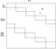
6.2 After row permutation. . . 52
6.3 The distribution of different types of non-zeros. . . 57
7.1 Effective memory bandwidth of condensation method. . . 69
7.2 CUDA code for condensation method and determinant on NTL over finite field. . . 71
7.3 CUDA code for condensation method and determinant on MAPLE over finite field. . . 71
8.1 Dividing the work of coefficient multiplication among threadblocks. . 81
9.1 A naive division step. . . 90
9.2 Optimize division steps. . . 93
9.3 Comparison between parallel plain division on CUDA and fast division in NTL for univariate polynomials with large degree gap. . . 95
9.4 Comparison between parallel GCD on CUDA and FFT-based GCD in NTL for univariate polynomials, with the same degree (n=m). . . . 102
10.2 Our GPU implementation versus FLINT for FFT-based polynomial
multiplication. . . 126
10.3 Evaluation lower degrees . . . 127
10.4 Evaluation higher degrees . . . 127
10.5 Interpolation lower degrees . . . 128
List of Tables
2.1 Work, span and parallelism of classical algorithms. . . 15
3.1 Algorithm parameters . . . 23
4.1 CPU times in seconds for both classical and cache-oblivious counting sort algorithm. . . 34
6.1 Test matrices with the number of non-zeros of typeα,β and δ. . . 60
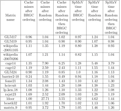
6.2 Normalized cache misses on ideal cache model simulator and normal-ized CPU time for SpMxVs. . . 61
6.3 Preprocessing time. . . 62
7.1 Determinant of Hilbert matrix by MAPLE, MATLAB, and condensa-tion method on both CPU and GPU. . . 74
7.2 Time(s) required to compute determinant of Hilbert Matrix by MAPLE, MATLAB, and condensation method on both CPU and GPU. 75 8.1 Long multiplication (n =m = 5). . . 78
8.2 Comparison between plain and FFT-based polynomial multiplications for balanced pairs (n=m) on CUDA. . . 84
8.3 Computation time for plain multiplication on CUDA for unbalance pairs (n6=m). . . 84
9.1 GCD implementation on CUDA with two different values of s. . . 101
10.1 Computation time for random polynomials with different degrees (2K) and points. All of the times are in seconds. . . 125
10.2 Execution times of multiplication . . . 125
10.3 Execution times of polynomial evaluation and interpolation. . . 126
Chapter 1
Introduction
This thesis deals with the implementation of basic routines in computer algebra tar-geting multi-core and many-core architectures. We consider routines from linear algebra (sparse and dense) and polynomial system solving. In contrast to their coun-terpart in numerical computing, these routines perform calculations in an exact and complete way. As a consequence, they are highly demanding in computer resources, time and memory. This often limits the impact of computer algebra software to problems of moderate size. However, the abundant computing power of hardware acceleration technologies suggests that much harder problems could be attacked with symbolic computation.
With respect to standard high-performance computing challenges, computer alge-bra low-level routines fall into the following categories.
(P1): Memory access patterns are highly irregular and work count is essentially pro-portional to the number of memory accesses. Typical examples are sparse ma-trix arithmetic and sparse polynomial arithmetic.
(P2): The amount of work is much larger than the amount of reads/writes while memory access patterns are rather regular. Typical examples are dense matrix arithmetic and dense polynomial arithmetic. While these routines allow for fine grain parallelism, certain complex memory access patterns (like for Fast Fourier Transform algorithms) make these operations not so suitable for multi-cores.
Problems of the first kind are more suitable for multicore architectures while problems of the second kind are eligible for many-core accelerators (like Graphics Processing Units).
multi-cores, we consider operations that are not suitable for many-multi-cores, due to large data size (a frequent issue in computer algebra) and that pause challenges in terms of memory transfer. For such operations, we propose pre-processing techniques that reshape the input data so as to reduce memory transfer when those operations are applied to the reshaped data. Cache complexity analysis and experimentation confirm the effectiveness of the proposed techniques. To be more specific, our work is driven by classical problem from linear algebra: improving data locality in sparse matrix vector (SpMxV) multiplication. This problem is hard as the permutation of rows or columns of a sparse matrix to maximize locality in SpMxV multiplication is NP-hard [59]. In Chapter 6, we propose a reordering algorithm for sparse matrices that improves the data locality during (SpMxV) multiplication. In each test-case, we re-arrange the input data and show that the cost of this re-arrangement can be amortized against the cost of calculations with the input data, such as linear system solving by iterative methods (conjugate gradient, etc.). We provide cache complexity analysis whose favorable results are confirmed experimentally. As a by-product of this research, we propose a new integer sorting algorithm, which is suitable for large sparse objects. This algorithm is described in Chapter 5.
On many-cores, we consider operations that are both data intensive and compute intensive, which is another frequent feature of computer algebra calculations, as men-tioned above. For such operations, we propose a computational model for designing algorithms targeting many-cores, with a focus on reducing parallelism overheads. We present a model of multithreaded computation namely many-core machine model (in Chapter 3) that combines the fork-join and SIMD parallelisms, with an emphasis on estimating parallelism overheads, so as to reduce scheduling and communication costs in GPU programs. We have applied this model and successfully reduced par-allelism overheads for several basic routines in polynomial algebra. For polynomial multiplication, our theoretical analysis allows us to reduce parallelism overheads due not only to data transfer but also to code divergence, see Chapter 8. For the Eu-clidean algorithm, our running time estimates match those obtained with the Systolic VLSI Array Model ([9]). Meanwhile, our CUDA code implementing this optimized Euclidean algorithm runs within the same estimate analyzed by our model for input polynomials with degree up to 100,000. This is reported in Chapter 9.
tree. For subproduct-tree operations, we demonstrate the importance of adaptive al-gorithms. That is, algorithms that adapt their behavior to the available computing resources. In particular, we combine parallel plain arithmetic and parallel fast arith-metic.
In Chapter 7, we present a GPU implementation of the condensation method for computing the determinant of a matrix. To the best of our knowledge, this is the first study of the parallelization of this algorithm. We consider both matrices with finite field coefficients and floating point number coefficients. Notably, the latter case exhibits favorable behavior in terms of numerical stability.
Chapter 2
Background
Until the advent of multi-core and many-core architectures, algorithms subject to effective implementation on personal computers were often designed with algebraic
complexity as the main complexity measure and with sequential running time as
the main performance counter [40, 41, 42, 13, 20]. Nevertheless, during the past 40 years, the increasing gap between memory access time and CPU cycle time, in favor of the latter, brought another important and practical efficiency measure: cache
complexity[36, 17]. In addition, with parallel processing becoming available on every
desktop or laptop, the work and span of an algorithm expressed in the fork-join multithreaded model [18, 13] have become the natural quantities to compute in order to estimate parallelism.
These complexity measures (algebraic complexity, cache complexity, parallelism) are defined for computation models that largely simplify reality. On many-core archi-tectures, several phenomena (parallelism overhead, synchronization among threads of all thread blocks, utilization of all multiprocessors, etc.) limit the performances of applications which, theoretically, have a lot of opportunities for concurrent execution.
2.1
Random access machine (RAM) model
can be programmed in some specified but arbitrary programming language. Some of the properties of this model are as follows:
• Each “simple operation” like addition, subtraction, multiplication, assign, branching, calling, etc. takes exactly 1 time step.
• Loops and procedures are considered to be the composition of many single-step operations.
• Each memory access takes exactly one time step, and we have as much memory as we need. The RAM model takes no notice of whether an item is in cache or on the disk, which simplifies the analysis.
A common problem of this model is that it is too simple, that is, these assumptions make the conclusions and analysis too hard to believe in practice. For instance, multiplying two numbers does not have the same cost as adding two numbers, which clearly violates the first assumption of the model. Memory access times also differ greatly depending on whether data are available in cache or on memory or on the disk, which violates the third assumption. However, in spite of having such restrictions, this model does not provide misleading results for the real world problems, since this only assumes a simple abstract model of computation. Furthermore, robustness of the RAM model enables us to analyze algorithms in a machine-independent way.
2.2
The PRAM model
The Parallel Random Access Machine (PRAM) is a natural generalization of RAM.
It has unbounded number of processors P0, P1, P2,· · ·. Each of these processors has
unbounded private local memory, which is a sets of registers. Unlike RAM model, it does not have tapes. The computing capability of each processor is the same as RAM. These processors can communicate with each other via shared memory (global
memory) M[0], M[1], M[2],· · · , which is also unbounded. Note that, it is the only
way, by which a processor can communicate with another processor. Each processor can access shared memory in unit time, unless there is a conflict.
In Figure 2.1, a PRAM model is shown. The input of a PRAM program consists of n items stored inM[0], . . . , M[n−1]. The output of a PRAM program consists of
n′ items stored inn′ memory cells, sayM[n], . . . , M[n+n′−1]. A PRAM instruction
executes in a 3-phase cycle:
1. Read (if needed) from a shared memory cell,
Figure 2.1: The PRAM model.
3. Write in a shared memory cell (if needed).
All processors execute their 3-phase cyclessynchronously. ProcessorP0 has a
spe-cialactivation registerspecifying the maximum index of an active processor. Initially,
onlyP0 is active; it computes the number of required active processors and loads this
number in the activation register. Then the corresponding processors start executing their programs. Computations proceed until P0 halts, at which time all other active
processors are halted.
The PRAM Model is attractive for designing parallel algorithms because of the following reasons.
• It is natural: the number of operations executed per one cycle on p processors is at most p.
• It is strong: any processor can read or write any shared memory cell in unit time.
• It is simple: ignoring any communication or synchronization overhead.
2.2.1
Parallel time, efficiency and speedup factor
The Parallel Time, denoted byT(n, p), is the time elapsed from the start of a parallel
computation to the moment where the last processor terminates, on an input data of size n, and using p processors. T(n, p) takes into account computational steps (such as adding, multiplying, swapping variables), routing (or communication) steps (such as transferring and exchanging information between processors). The parallel
efficiency, denoted byE(n, p), is
E(n, p) = SU(n)
pT(n, p),
where SU(n) is a lower bound for a sequential execution. Observe that we have
SU(n)≤p T(n, p) and thus E(n, p)≤1. One also often considers the speedup factor
defined by
S(n, p) = SU(n)
T(n, p).
2.2.2
Different types of PRAM models
It is natural to have conflicts in accessing shared memory for some applications. To resolve this issue and synchronize the parallel execution, some mechanism has to be defined for concurrent read and write access conflicts to the same shared memory cell. Some of the basic submodels of PRAM are given below.
Exclusive Read Exclusive Write (EREW). No two processors are allowed to read or write the same shared memory cell simultaneously.
Concurrent Read Exclusive Write (CREW).Simultaneous reads of the same mem-ory cell are allowed, but no two processors can write the same shared memmem-ory cell simultaneously.
Concurrent Read Concurrent Write (CRCW). Simultaneous reads and writes of the same memory cell are allowed. CRCW can be divided further based on concurrent writes.
PRIORITY Concurrent Read Concurrent Write (PRIORITY CRCW).
Simul-taneous reads of the same memory cell are allowed. Processors are assigned fixed and distinct priorities. In case of write conflict, the processor with highest priority is allowed to complete WRITE.
ARBITRARY Concurrent Read Concurrent Write (ARBITRARY CRCW).
f
athena,cel,prokop,sridhar
g@supertech.lcs.mit.edu
= ( )
( + = )
( +( = )( + )) ( )
( +( + + )= + =
p )
( ; )
Q
cache
misses
organized by
optimal replacement
strategy
Main
Memory
Cache
Z
=L Cache lines
Lines
of length L
CPU
W
work
>
= ( );
( )
Figure 2.2: The ideal-cache model.
randomly chosen processor is allowed to complete WRITE. An algorithm written for this model should make no assumptions about which processor is chosen in case of write conflict.
COMMON Concurrent Read Concurrent Write (COMMON CRCW).
Simul-taneous reads of the same memory cell are allowed. In case of write conflict, all processors are allowed to complete WRITE iff all values to be written are equal. An algorithm written for this model should make sure that this condition is satisfied. If not, the algorithm is illegal and the machine state will be undefined.
2.3
The ideal cache model
The cache complexity of an algorithm aims at measuring the (negative) impact of
memory traffic between the cache and the main memory of a processor executing that algorithm. Cache complexity is based on the ideal-cache model shown in Figure 2.2. This idea was first introduced by Matteo Frigo, Charles E. Leiserson, Harald Prokop, and Sridhar Ramachandran in 1999 [17]. In this model, there is a computer with a two-level memory hierarchy consisting of an ideal (data) cache of Z words and an arbitrarily large main memory. The cache is partitioned into Z/L cache lines where
L is the length of each cache line representing the amount of consecutive words that are always moved in a group between the cache and the main memory. In order to achieve spatial locality, cache designers usually use L >1 which eventually mitigates
the overhead of moving the cache line from the main memory to the cache. As a result, it is generally assumed that the cache is tall and practically that we have
Z = Ω(L2).
In the sequel of this thesis, the above relation is referred as thetall cache assumption. In the ideal-cache model, the processor can only refer to words that reside in the cache. If the referenced line of a word is found in cache, then that word is delivered to the processor for further processing. This situation is literally called a cache hit. Otherwise, a cache miss occurs and the line is first fetched into anywhere in the cache before transferring it to the processor; this mapping from memory to cache is called full associativity. If the cache is full, a cache line must be evicted. The ideal cache uses the optimal off-line cache replacement policy to perfectly exploit temporal
locality. In this policy, the cache line whose next access is furthest in the future is
replaced [5].
Cache complexity analyzes algorithms in terms of two types of measurements. The first one is thework complexity,W(n), wherenis the input data size of the algo-rithm. This complexity estimate is actually the conventional running time in a RAM model [1]. The second measurement is its cache complexity, Q(n;Z, L), representing the number of cache misses the algorithm incurs as a function of:
• the input data size n, • the cache size Z, and
• the cache line length L of the ideal cache.
When Z and L are clear from the context, the cache complexity can be denoted simply by Q(n).
An algorithm whose cache parameters can be tuned, either at compile-time or at runtime, to optimize its cache complexity, is called cache aware; while other al-gorithms whose performance does not depend on cache parameters are called cache
oblivious. The performance of cache-aware algorithm is often satisfactory. However,
there are many approaches which can be applied to design optimal cache oblivious algorithms to run on any machine without fine tuning their parameters.
B
B
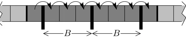
Figure 2.3: Scanning an array of n=N elements, with L=B words per cache line.
from the external-memory bound [36]. However, such type of error is reasonable as our main goal is to match bounds within multiplicative constant factors.
Proposition 1. Scanning n elements stored in a contiguous segment of memory with
cache line size L costs at most ⌈n/L⌉+ 1 cache misses.
Proof⊲The main ingredient of the proof is based on the alignment of data elements
in memory. We make the following observations.
• Let (q, r) be the quotient and remainder in the integer division of n byL. Let
u (resp. w) be the total number of words in a fully (not fully) used cache line. Thus, we have n=u+w.
• If w = 0 then (q, r) = (⌊n/L⌋,0) and the scanning costs exactly q; thus the conclusion is clear since⌈n/L⌉=⌊n/L⌋ in this case.
• If 0< w < L then (q, r) = (⌊n/L⌋, w) and the scanning costs exactlyq+ 2; the conclusion is clear since⌈n/L⌉=⌊n/L⌋+ 1 in this case.
• If L ≤ w < 2L then (q, r) = (⌊n/L⌋, w −L) and the scanning costs exactly
q+ 1; the conclusion is clear again.
⊳
2.4
The multi-core machine model
The cores in a multi-core architecture can be connected tightly or loosely. For in-stance, cores may or may not share caches, and they may implement inter-core com-munication techniques such as message passing or shared memory. Common network topologies are used to interconnect cores, including bus, ring, two-dimensional mesh and crossbar. Homogeneous multi-core systems include only identical cores, whereas,
heterogeneousmulti-core systems have cores which are not identical in practice. Cores
on multi-ore systems may implement architecture features such as instruction level parallelism (ILP), vector processing, SIMD or multithreading, similar to those of single-processor systems.
The advantages of multi-core architecture include the fact that cache coherency
circuitry operates at a much higher clock-rate than in distributed systems where the signals have to travel off-chip. That is, signals between different CPUs (cores) travel shorter distances, and therefore those signals degrade less. As a result, these higher-quality signals with high frequency allow more data to be transferred within a short time period. Moreover, a multi-core processor usually uses less power than multiple coupled single-core processors, this is because of the reduced power required to drive off-chip signals. Furthermore, the cores share some circuitry, like the L2 cache and the interface to the front side bus (FSB). Also, multi-core design produces a product with lower risk of design error than devising a new wider core-design.
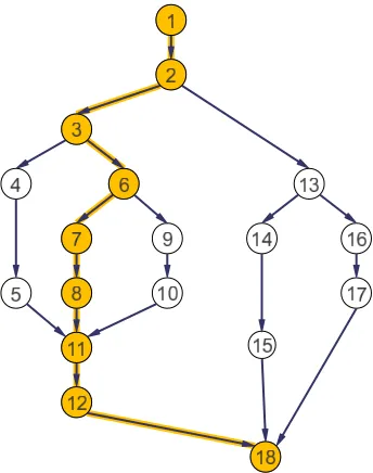
Figure 2.4: A directed acyclic graph (dag) representing the execution of a multi-threaded program. Each vertex represents an instruction while each edge represents a dependency between instructions.
2.5
The fork-join parallelism model
TheCilk++1 concurrency platform [7, 18, 45, 15] provides a simple theoretical model called the fork-join parallelism model or dag (direct acyclic graph) model of threading for parallel computation. This model represents the execution of a multi-threaded program as a set of nonblocking threads denoted by the vertices of a dag, where the dag edges indicate dependencies between instructions. See Figure 2.4.
In the Cilk++ terminology, a thread is a maximal sequence of instructions that ends with a spawn, sync, orreturn statement. These statements are used to denote respectively:
• anexecution flow forking,
• a synchronization point, at which currently running threads must join before
the execution flow proceeds further, • the return point of a function.
A correct execution of a Cilk++ program must meet all the dependencies in the dag, that is, a thread cannot be executed until all the depending treads have com-pleted. The order in which these dependent threads will be executed on the processors is determined by the scheduler.
1
Cilk++s scheduler executes anyCilk++computation in a nearly optimal time, see [18] for details. From a theoretical viewpoint, there are two natural measures that allow us to define parallelism precisely, as well as to provide important bounds on performance and speedup which are discussed in the following subsections.
2.5.1
The work law
The first important measure is thework which is defined as the total amount of time required to execute all the instructions of a given program. For instance, if each instruction requires a unit amount of time to execute, then the work for the example dag shown in Figure 2.4 is 18.
Let TP be the fastest possible execution time of the application on P processors. Therefore, we denote the work by T1 as it corresponds to the execution time on 1
processor. Moreover, we have the following relation
Tp ≥T1/P, (2.1)
which is referred as thework law. In our simple theoretical model, the justification of this relation is easy: each processor executes at most 1 instruction per unit time and therefore P processors can execute at most P instructions per unit time. Therefore,
the speedup onP processors is at most P since we have
T1/TP ≤P. (2.2)
2.5.2
The span law
The second important measure is based on the program’scritical-path lengthdenoted by T∞. This is actually the execution time of the application on an infinite number
of processors or, equivalently, the time needed to execute threads along the longest path of dependency. As a result, we have the following relation, called the span law:
TP ≥T∞. (2.3)
2.5.3
Parallelism
In the fork-join parallelism model,parallelismis defined as the ratio of work to span, orT1/T∞. Thus, it can be considered as the average amount of work along each point
greater thanT1/T∞. Indeed, Equations 2.2 and 2.3 imply that speedup satisfies
T1/TP ≤T1/T∞≤P.
As an example, the parallelism of the dag shown i n Figure 2.4 is 18/9 = 2. This means that there is little chance for improving the parallelism on more than 2 processors, since additional processors will often starve for work and remain idle.
2.5.4
Performance bounds
For an application running on a parallel machine withP processors with workT1 and
span T∞, the Cilk++ work-stealing scheduler achieves an expected running time as
follows:
TP =T1/P +O(T∞), (2.4)
under the following three hypotheses: • each strand executes in unit time,
• for almost all parallel steps there are at least p strands to run, • each processor is either working or stealing.
See [18] for details.
If the parallelismT1/T∞is so large that it sufficiently exceeds P, that isT1/T∞≫
P, or equivalentlyT1/P ≫T∞, then from Equation (2.4) we haveTP ≈T1/P. From
this, we easily observe that the work-stealing scheduler achieves a nearly perfect linear speedup of T1/TP ≈P.
2.5.5
Work, span and parallelism of classical algorithms
The work, span and parallelism of some of the classical algorithms in the fork-join parallelism model is shown in Table 2.1.
2.6
Systolic arrays
Algorithm Work Span Parallelism Merge sort Θ(n log2(n)) Θ(log2(n)3) Θ(log2n(n)2)
Matrix multiplication Θ(n3) Θ(log
2(n)) Θ( n
3
log2(n))
Strassen Θ(nlog2(7)) Θ(log
2(n)2) Θ(n
log2(7)
log2(n)2)
LU-decomposition Θ(n3) Θ(n log
2(n)) Θ( n
2
log2(n))
Tableau construction Θ(n2) Ω(nlog2(3)) Θ(n0.415)
FFT Θ(n log2(n)) Θ(log2(n)2) Θ( n
log2(n))
Table 2.1: Work, span and parallelism of classical algorithms.
Matrix multiplication might be a good example of the design of systolic algorithm, where one matrix is fed in a row at a time from the top of the array and is passed down the array. The other matrix is fed in a column at a time from the left hand side of the array and passes from left to right. In order to be seen each processor as a whole row and a whole column, dummy values are often passed in when they are not like so. Finally, the multiplication result is stored in the array and can now be output a row or a column at a time, flowing down or across the array.
Lots of applications of systolic arrays include faster input processing, scalability, high throughput etc. The cells are organized in such a way that it can simultaneously process the input, that is, its processing is faster than the conventional computing architecture. Also, this architecture can easily be extended to many more processors according to the requirements of the application. Moreover, systolic arrays offer a way to take certain exponential algorithms and use hardware to make them linear.
Chapter 3
Many-core Machine Model
We propose a model of computations which aims at capturing parallelism overheads (such as communication and synchronization costs) of programs written for modern GPU architectures. We establish a Graham-Brent theorem for this model so as to estimate running time of programs running on p streaming multiprocessors. We evaluate the benefits of our model with three applications. In each case, our model is used to optimize a program parameter controlling overhead.
This chapter is a joint work with M. Moreno Maza and N. Xie.
3.1
Introduction
Designing efficient algorithms targeting implementation on hardware accelera-tion technologies (multi-core processors, graphics processing units (GPUs), field-programmable gate arrays) creates major challenges for computer scientists. A first difficulty is to define models of computations retaining the features of actual comput-ers that have a dominant impact on program performance. This implies to specify not only the appropriate complexity measures for algorithms but also the relevant parameters for the theoretical machine executing those algorithms. Once different algorithmic solutions for a given problem and a given model of computations are available, a second difficulty is to combine those complexity measures in order to select the “best” algorithm.
variant of this latter theorem is actually supporting successfully the implementation of the parallel performance analyzer calledCilkview[35] on multi-core architectures. With many-core processors, in particular GPUs, one needs to integrate SIMD (Single Instruction Multiple Data) processing into the model. The PRAM model ([66, 22]) has this flavor but it does not have the task-parallelism dimension which is necessary to represent the relations between the different kernels of an application written with the Compute Unified Device Architecture (CUDA) [58]. In addition, the PRAM model fails to retain important features of actual computers related to memory traffic, such as cache complexity ([18, 19]). This latter notion has been proved to be very useful on single-core and multi-core multiprocessors.
An attempt to integrate memory contention into the PRAM model has been made with the QRQW (Queue Read Queue Write) PRAM, defined in [23] by Gibbons, Matias and Ramachandran. The Authors also enhance the Graham-Brent theorem. However, they unify in a single quantity time spent in arithmetic operations and time spent in read/write accesses. We believe that this unification is not appropriate for recent many-core processors, such as GPUs, for which the ratio between one read/write access to the global memory and one floating point operation can be in the 100’s.
In a recent paper, Ma, Agrawal and Chamberlain [48] introduce the TMM (Threaded Many-core Memory) model which retains many important characteristics of GPU-type architectures, including several machine parameters such as throughput and coalesced granularity. Moreover, while their running time estimate onP cores is not a Graham-Brent theorem, TMM analysis can order algorithms from slow to fast for many different settings of those machine parameters.
Many works, such as [49, 47], targeting code optimization and performance pre-diction of GPU programs are related to our work, though these papers do not define an abstract model in support of algorithm analysis.
In this chapter, we propose a many-core machine model (MMM) which aims at optimizing algorithms targeting implementation on GPUs. We insist on the following aspects:
- Two-level DAG programs. Defined in Section 3.2, this feature captures the two
levels of parallelism (fork-join and SIMD) of CUDA-like programs.
- Parallelism overhead. We introduce this complexity measure in Section 3.2.3
with the objective of analyzing communication and synchronization costs.
and parallelism overhead) and two machine parameters (size of local memory and data transfer throughput) in order to estimate the running time of an MMM program on p streaming multiprocessors. This result is Theorem 1 in Section 3.2.4.
To demonstrate and evaluate the benefits of our model, we consider three applica-tions for which we have realized an implementation reported in [31]. In each case, the parallelism overhead (and also the work, to a lesser extent) depends on a pro-gram parameter. For the first two applications, namely polynomial division and the Euclidean Algorithm (see Chapter 9),
this parameter controls the amount of data transfer between global memory and local memories. For the third application, polynomial multiplication (see Chapter 8) this parameter controls the amount of branch divergence (see [25] for optimization techniques related to this performance issue) which can also be seen as a parallelism overhead.
For each of these three applications, we apply the following strategy.
1. We determine a value of this program parameter that minimizes parallelism overhead.
2. We check that the work overhead introduced by this optimization technique remains very low. In fact, this work overhead is typically 30% of the work of the non-optimized algorithm.
3. We use our version of Graham-Brent theorem to show that the estimated run-ning time (onpstreaming multiprocessors) of the optimized algorithm is asymp-totically smaller than that of the non-optimized algorithm. In fact, this speedup is typically a factor of 2, which is confirmed by the experimental study of [31].
Finally, we observe that, in our model, the Euclidean Algorithm reaches the running estimates predicted by the Systolic VLSI Array Model [9]. At the same time, the CUDA code implementing the Euclidean Algorithm developed with our model runs within the same estimate for input polynomials with degree up to 100,000, as reported in [31].
3.2
A many-core machine model
with low latency and high throughput. One of the main reasons for this optimization is the fact that global memory latency is approximately 400 to 800 cycles, while lo-cal memory latency is only a few cycles. This memory latency difference, when not properly taken into account, may have a dramatic negative impact on program per-formance. As mentioned in the introduction, this hardware feature of GPUs cannot be captured by the well-studied PRAM model. Indeed, any memory access, as well as any integer arithmetic operation, is performed in unit time on a PRAM machine. This and other limitations of the PRAM model have motivated variants of this model, including our work. Another motivation is the new programming model sup-ported by NVIDIA1 Kepler architecture, which allows algorithms to run entirely on the device (GPU) without host (CPU) interactions. The model of parallel computa-tions presented in this paper aims at capturing communication and synchronization overheads of programs written for modern GPU architectures, such as NVIDIA Fermi and NVIDIA Kepler.
As specified in Sections 3.2.1 and 3.2.2 below, our many-core machine model (MMM) retains many of the key characteristics of modern GPU architectures and the CUDA programming model. However, in order to support algorithm analysis, with an emphasis on parallelism overheads, as defined in Section 3.2.3, an MMM machine admits a few simplifications and limitations with respect to an actual GPU device. We justify those choices in Section 3.2.5 and explain how more general models can be reduced to ours.
3.2.1
Many-core machine characteristics
Architecture. An MMM machine possesses an unbounded number ofstreaming
mul-tiprocessors(SMs) which are all identical. Each SM has a finite number of processing
cores and a fixed-size local memory. An MMM machine has a 2-level memory hierar-chy, comprising an unbounded global memory with high latency and low throughput while the SM local memories have low latency and high throughput.
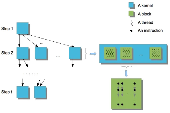
Programs. An MMM program is a directed acyclic graph (DAG) whose vertices are kernels and where edges indicate dependencies, similarly to the instruction stream DAGs of the fork-join multithreaded parallelism model [6]. Akernelis a SIMD (single instruction multithreaded data) program decomposed into a number of thread-blocks.
Each thread-block is executed by a single SM and each SM executes a single
thread-block at a time. Similarly to a CUDA program, an MMM program specifies for each
1
Figure 3.1: Overview of a many-core machine program
kernel call the number of thread-blocks and the number of threads per thread-block. The different types of components of an MMM program are depicted on Figure 3.1.
Scheduling and synchronization. At run time, an MMM machine schedules thread-blocks (from the same or different kernels) onto SMs, based on (1) the dependencies specified by the edges of the DAG and, (2) the hardware resources required by each thread-block. Threads within a thread-block can cooperate with each other via the local memory of the SM running the thread-block. Meanwhile, thread-blocks interact with each other via the global memory. In addition, threads within a thread-block are executed physically in parallel by an SM. Meanwhile, the programmer cannot make any assumptions on the order in which thread-blocks of a given kernel are mapped to the SMs. This restriction allows MMM programs to run correctly on any fixed number of SMs, similarly to a CUDA program.
Memory access policies. All threads of a given thread-block can access simultane-ously any memory cell of the local memory or the global memory: read/write conflicts are handled by the CREW (concurrent read and exclusive write) policy. However, read/write requests to the global memory by two different thread-blocks cannot be executed simultaneously. In case of simultaneous request, one thread-block is chosen randomly and served first, then the other thread-block is served.
For the purpose of analyzing program performance, we define two machine
pa-rameters:
Z: Size (expressed in machine words) of the local memory of each SM.
To be precise, the throughput 1/U satisfies the following property. Ifrand ware the number of words respectively read and written to the global memory by one thread of a thread-block B, then the total timeTD spent in data transfer between the global memory and the local memory of an SM executing B satisfies
TD ≤(r+w)U. (3.1)
We observe that most phenomena that ease or limit data transfer (coalesced accesses to global memory, local memory bank conflicts, partition camping, etc) have an im-pact on running time which is proportional to the amount of transferred data. This allows us to claim that the throughput 1/U combines (or unifies) these different phe-nomena.
Similarly, the local memory sizeZ unifies in one parameter different characteristics of an SM and, thus, of a thread-block. Indeed, each of the following quantities is necessarily at most equal toZ: the number of cores of an SM, the number of threads of a thread-block, the amount of words in a data transfer between the global memory and the local memory of an SM.
Relation (3.1) calls for another comment. One could expect the introduction of a third machine parameter, say V, such that, if ℓ is the number of local operations
(arithmetic operations, reads/writes in the local memory) performed by one thread of the thread-block B, then the total time TA spent in local operations by an SM executing B would satisfy
TA ≤ℓV. (3.2)
As a consequence, for the total running timeT of the thread-block B, we would have
T =TA+TD ≤ℓV + (r+w)U. (3.3)
Instead of introducing this third machine parameter V, we let V = 1, which is equivalent to a change of coordinates.
3.2.2
Many-core machine programs
be precise, a kernel call can be executed provided that all its predecessors in the DAG (K,E) have completed their execution.
Recall that each kernel decomposes into one or more thread-blocks and that all threads within a given kernel execute the same serial program, but with possibly differ-ent input data. In addition, all threads within a thread-block are executed physically in parallel by an SM. It follows that MMM kernel code needs no synchronization statement, like CUDA’s syncthreads().
This has two consequences. First, each thread in a thread-block is either submit-ting read/write requests to the global memory or, execusubmit-ting local operations. This justifies Relation (3.3). A second consequence is the fact that the synchronization overheads of an MMM program are included in the scheduling costs of the thread-blocks onto the SMs. We shall assume that those latter costs depend linearly on the number of thread-blocks and the sum over all thread-blocks of the amount of data transferred by one thread. Indeed, this second quantity can be used to estimate the size of the code of a thread-block. Therefore, synchronization overheads of an MMM program can be incorporated in the data transfer time. This key observation helps understanding the complexity measures introduced in Section 3.2.3.
Since each kernel of the program P decomposes into a finite number of thread-blocks, we map P to a second graph, called the thread block DAGof P, whose vertex setB(P) consists of all thread-blocks of the kernels ofP and such that (B1, B2) is an
edge if B1 is a thread-block of a kernel preceding the kernel of B2 inP. This second
graph is associated two important quantities:
N(P): number of vertices in the thread-block DAG of P,
L(P): critical path length (that is, the length of the longest path) in the thread-block DAG of P.
For the purpose of analyzing program performance, we define fiveprogram
param-eters, summarized in Table 3.1.
Parameter Description
n Input size in machine words
z Maximum number of words of local memory allocated per thread-block
q The number of threads per thread-block
d The maximum number of thread-blocks in a parallel step
π The number of parallel steps
Table 3.1: Algorithm parameters
3.2.3
Complexity measures for the many-core machine
model
Consider, as before, an MMM programP given by its kernel DAG (K,E). LetK ∈ K
be any kernel ofP andB be any thread-block ofK. We define theworkofB, denoted byW(B), as the total number of local operations performed by the threads ofB. We define the span of B, denoted by S(B), as the maximum number of local operations performed by a thread of B. We assume that each thread of B reads r words and writesw words from the global memory. Then, we define theoverheadof B, denoted by O(B), as (r+w)U. The work W(K) of the kernel K is defined as the sum of the works of its thread-blocks. The span (resp. overhead) S(K) (resp. O(K)) of the kernelK is defined as the maximum (resp. sum) of the spans (resp. overheads) of its thread-blocks.
We consider now the entire program P. The work W(P) of P is defined as the total work of all its kernels
W(P) = X K∈K
W(K).
Regarding the graph (K, E) as a weighted-vertex graph where the weight of a vertex
K ∈ K is its span S(K), we define the weight S(γ) of any path γ from the first executing kernel to a last executing kernel as
S(γ) = X K∈γ
S(K).
Then, we define the spanS(P) of the program P as
Regarding the graph (K, E) as a weighted-vertex graph, where the weight of a vertex
K is its overheadO(K), we define the overheadO(α) of an anti-chainα of (K, E) as
O(α) = X K∈α
O(K),
Finally, we define the overheadO(P) of P as the sum of the O(α)’s among all anti-chains α in (K, E), that is,
O(P) = X α
O(α).
Observe that, according to Mirsky’s theorem [50], the numberπof parallel steps inP (i.e. anti-chains in (K,E)) is equal to the maximum length of a path in (K,E) from the first executing kernel to a last executing kernel.
3.2.4
A Graham-Brent theorem with overhead
Theorem 1. We have the following estimate for the running timeTP of the program
P when executed on p SMs,
TP ≤(N(P)/p+L(P))C(P) (3.4)
where C(P) = maxB∈B(P)(S(B) +O(B)).
The proof is similar to that of the original result. One observes that the total number of complete steps (for which p thread-blocks can be scheduled by a greedy scheduler) is at most N(P)/pwhile the number of incomplete stepsis at most L(P). Finally, C(P) is an obvious upper bound for the running of every step, complete or incomplete.
3.2.5
Justification of the many-core machine model
Chapter 4
Cache-oblivious Counting Sort
Algorithm
In this chapter, we propose a cache-oblivious counting sort algorithm. Cache com-plexity estimates of both classical and our proposed cache-oblivious counting sort al-gorithm are provided considering the ideal cache model. We have implemented these algorithms and compared them by experimentation. Based on those cache complexity results and experimental results, we can say that our cache-oblivious counting sort algorithm is promising.
This chapter is a joint work with M. Moreno Maza.
4.1
Introduction
The counting sort algorithm sorts n non-negative integers in the range [0, r−1] in linear time with respect to n +r considering the RAM model [13]. Algorithm 1 describes the classical counting sort algorithm. Observe that the counting sort algo-rithm does not require a comparand function. Thus it does not have time complexity lower bound of the form O(nlogn) like any comparison based sorting algorithms.
In this chapter, time and space complexity are computed considering the RAM model with memory holding a finite number of s-bit words, for a fixed s [64]. We assume each of the integers to be sorted can be stored within one machine word. Our cache complexity results are computed considering the ideal cache model [17] with an ideal cache of Z words and for which each cache line holds L words.
sort algorithms. We validate theoretical results by experimentation. Similar work can be found in [61] but the Authors do not make use of the ideal cache model.
The organization of this chapter is as follows. we first describe the classical count-ing sort algorithm along with its cache complexity in Section 4.2. We then present our cache-oblivious counting sort algorithm along with its cache complexity in Section 4.3 followed by experimental results in Section 4.4. We conclude the chapter with some remarks on our approach.
4.2
The classical counting sort algorithm
Algorithm 1 is the classical counting sort algorithm. Proposition 2 computes the cache complexity of this algorithm.
Algorithm 1: CountingSort(A, n, r)
Input: A is an array of length n that holds n integers in the range [0, r−1].
Output: Array B of lengthn, where the integers in A are sorted. initialize an array C of length r of with zeros;
1
for i= 0;i < n;i=i+ 1 do
2
C[A[i]] =C[A[i]] + 1; 3
t = 0; 4
for i= 0;i < r;i=i+ 1 do
5
c=C[i]; 6
C[i] =t; 7
t =t+c; 8
for i= 0;i < n;i=i+ 1 do
9
B[C[A[i]]] =A[i]; 10
C[A[i]] =C[A[i]] + 1; 11
return B; 12
Proposition 2. Given an array A of length n that holds n non-negative integers
within the range [0, r−1], the total number of cache misses in Algorithm 1 is at most
3n+ 2n/L+ 2r/L+ 4, where both n and r are small enough such that none of A or
B or C can be stored into the cache entirely.
Proof ⊲We follow the pseudo-code of Algorithm 1 and count the number of cache misses.
Initializing C with zeros in line 1: This involves traversingC in a regular way (i.e. one
Computing frequency of the integers ofA intoC in lines 2-3: This involves traversing
A in a regular way. However, C is accessed n times in an irregular way. So the total number of cache misses is (n/L+ 1) +n in the worst case. The latter n cache misses are due to both capacity and conflict misses in accessing C irregularly.
Computing the cumulative frequency in C in lines 5-8: This involves traversing C in
a regular way, thus causing r/L+ 1 cache misses.
Creating sorted arrayB in lines 9-11: Finally, populating the sorted arrayB involves
traversing the three arraysA,B and C. The arrayAis accessed in a regular fashion. However, the n accesses to C and B are irregular. So the total number of cache misses is (n/L+ 1) + 2n in the worst case. The latter 2ncache misses are due to both capacity and conflict misses in accessing C and B irregularly.
Irregular access make the performance of counting sort algorithm poor in terms of cache misses, for largen orr, as we can see in Section 4.4. In Section 4.3, we propose a cache-oblivious counting sort algorithm in order to reduce the cache complexity of this algorithm.
4.3
Cache-oblivious counting sort algorithm
In Proposition 3, we first estimate the number of cache misses of Algorithm 1 with small r. This leads us to the notion of a bucketed array introduced in Definition 1. We show the cache complexity is reduced during counting sort algorithm if the input
A has this property. Finally, we propose a preprocessing step (Algorithm 2) which rearranges the integers in A in such a way that it can be bucketed.
Proposition 3. The cache complexity of Algorithm 1 is at most 3n/L+r+r/L+ 3
for r < Z/(1 +L), where n is small enough such that none of A or B can be stored into the cache entirely.
In lines 9-11, the cache misses due to accessing A exhibit the same cache com-plexity as described in the proof of Proposition 2. Writing sorted array B means writing (in a linear traversal) r consecutive arrays, of possibly different sizes, but with total size n. Thus, because of possible misalignments between those arrays and their cache-lines, this writing procedure can yield at most n/L+r cache misses (and not justn/L+ 1). It is possible if the ideal cache has at least r cache lines. We know the ideal cache has Z/L cache lines and we have r < Z/(1 +L) < Z/L. Observe C
is stored entirely into the cache before the algorithm enters line 9. To keepC stored entirely into the ideal cache during the execution of lines 9-11 and to observe at most
n/L+rcache misses for writing the sorted array B, we require an ideal cache where,
(r+rL)< Z. (4.1)
Equation 4.1 holds for our case, because dividing both sides by (1 +L) yields
r < Z/(1 +L).
From Proposition 3, we can say that counting sort is ideal for sorting integers with small range. The hypothesis of Proposition 3 leads us to introduce the following notion.
Definition 1. Given an array A of length n with non-negative integer entries in the
range [0, ℓm−1], where ℓ andm are positive integers. We say that A is m-bucketed
if for all i= 0,1· · · ,(ℓ−1), the integers in the sub-range [im,(i+ 1)m−1]are kept
together in A. In other words, for all j = 0,1· · · ,(ℓ−1), every integer of A lying in
the sub-range [jm,(j + 1)m−1] appears in A before every integer of A lying in the
sub-range [(j + 1)m, ℓm−1].
In Proposition 4, we estimate the cache complexity of the counting sort algorithm when the input array A ism-bucketed.
Proposition 4. Let the input array A be m-bucketed as described in Definition 1,
where m < Z/(1 +L). The cache complexity of Algorithm 1 is at most 3n/L+ 4r/L+
(m+ 2)ℓ+ 4, where n is small enough such that none of A or B can be stored into
the cache entirely.
Proof⊲Algorithm 1 initializesCwith zeros, computes cumulative frequencies inC
as described in the proof of Proposition 2. Moreover while counting the frequencies of the integers in lines 2-3 and creating the sorted array B in the last for-loop of the algorithm, the traversals ofAare also regular. Thus it has the same cache complexity as in the proof of Proposition 2. Together we have 2n/L+ 2r/L+ 4 cache misses for accessing A and C twice in a regular fashion.
For lines 2-3, accessing C for computing the frequency of the integers inA means traversing ℓ consecutive arrays one after another, of possibly different sizes (at most
m), but with total size r. In lines 9-11, we need to access C in the same fashion. Thus the total number of cache misses is at most 2r/L+ 2ℓ for accessing C in these two for-loops.
Let us consider a sub-range [im,(i+ 1)m−1] of A fori= 0,1· · · ,(ℓ−1). Letni be the total number of integers in this sub-range. From the proof of Proposition 3, we can say that, the cache complexity for writing into B due to this sub-range is at most ni/L+m. So in total we have at mostn/L+mℓcache misses for writing B. Now, we describe our cache-oblivious counting sort algorithm. Our proposed algorithm has a preprocessing step, stated in Algorithm 2. This algorithm calls Algo-rithm 3 iteratively. Assumption 1 below gathers two relations among the quantities
r, Z and L. The first one is made in a sake of simplicity. The second one is taken from Definition 1.
Assumption 1. We assume that r is of the form r =mu+1, for some non-negative
integer u and a positive integer m such that we have m < Z/(1 +L).
Algorithm 2: PreprocessingCounting(A, n, m, r)
Input: A is an array of lengthn holding non-negative integers in the range [0, r−1] andm is a positive integer as defined in Assumption 1.
Output: the array A which was overwritten such thatA is now m-bucketed.
r′ =r;
1
while r′ > m do
2
G= PartitionFurther(A, n, m, r, r′);
3
r′ =r′/m;
4
copy G into A; 5
return A; 6
The cache complexity of Algorithm 3 is given in Proposition 6.
Proof⊲For simplicity, we describe the proof for the first bucket. Consider the sub-array A[0. . . j], where 0 ≤ j < n, stores the first bucket or the sub-range [0, r′−1].
The first iteration of the top for-loop of Algorithm 3 is responsible for rearranging these integers such that A[0. . . j] is m-bucketed into G[0. . . j].
We follow the pseudo-code of Algorithm 2 for the first iteration and check its correctness. Observe each integer in A[0. . . j] is treated as an integer in the range [0, m−1] when we apply floor function after division in both line 9 and 16. In lines 8-10, we compute the frequency of integers in A[0. . . j] into F. In lines 11-14, we compute the cumulative frequencies in F as in lines 5-8 of Algorithm 1. Finally, in lines 15-19, we write into the sub-arrayG[0, . . . , j] asm-bucketed integers inA[0. . . j] with the help of F.
The other r/r′−1 iterations in Algorithm 2 can be proved in the same way.
Algorithm 3: PartitionFurther(A, n, m, r, r′)
Input: An array A of lengthn holdingn positive integers in the range [0, r−1] and a positive integer m as defined in Assumption 1. Moreover, the array A is assumed to be (r/r′)-bucketed.
Output: An array G of lengthn holding the samen entries as A but re-ordered in a such way such that G is ((r/r′)m)-bucketed.
y =r/r′;
1
d=r′/m;
2
create an array F of length m; 3
x= 0; 4
G is an array of length n; 5
for (i= 0;i < y;i=i+ 1) do
6
make all entries of F as 0; 7
for (j =x;j < n ∧ A[j]< r′(i+ 1);j =j+ 1) do
8
F[⌊(A[j]−r′i)/d⌋] =F[⌊(A[j]−r′i)/d⌋] + 1;
9
t = 0; 10
for (j = 0;j < m;j =j+ 1) do
11
c=F[j]; 12
F[j] =t; 13
t =t+c; 14
for (j =x;j < n ∧ A[j]< r′(i+ 1);j =j+ 1) do
15
k =⌊(A[j]−r′i)/d⌋;
16
G[F[k] +x] =A[j]; 17
F[k] =F[k] + 1; 18
x=x+ 1; 19
Proposition 6. In Algorithm 3, we can observe at most3n/L+m/L+(r/r′)(2+m)+1
cache misses, where n is small enough such that none of A or G can be stored into
the cache entirely.
Proof ⊲ We follow the pseudo-code of the algorithm and count the number of
cache misses during the first iteration of the top for-loop of Algorithm 3. Like the proof of Proposition 5, consider the sub-array A[0. . . j], where 0 ≤ j < n, stores the first bucket or the sub-range [0, r′ −1]. The first iteration of the top for-loop
of Algorithm 3 is responsible for rearranging these integers such that A[0. . . j] is
m-bucketed into G[0. . . j].
We first initialize F with zeros in line 7. This involves traversing F in a regular way. Thus, this causes m/L+ 1 cold misses. In lines 8-9, we compute the number of integers in A[0. . . j] that falls into each bucket. This involves traversingA[0. . . j] in a regular way. So the number of cache misses for accessing A[0. . . j] is at most
j/L+ 1 during this step. As m < Z/(1 +L), like in the proof of Proposition 3, we do not observe any cache misses for accessingF. For the same reason, we do not observe any cache misses for accessing F in the rest of the execution of this algorithm.
Finally, in lines 15-19, when we write the m-bucketed integers in G[0. . . j], we need to traverse A[0. . . j] in a regular fashion again. Moreover, we need to write the m-bucketed integers into G[0. . . j]. This refers to write (in a linear traversal) m
consecutive arrays, of possibly different sizes, but with total size j. From the proof of Proposition 3, we can say that the cache complexity for writing into G[0. . . j] is at most j/L+m. Thus the total number of cache misses for accessingA[0. . . j] and
G[0. . . j] in this iteration is at most 3j/L +m + 2. So the cache complexity for accessingA andGin Algorithm 3 is at most 3n/L+ (m+ 2)(r/r′), as the top for-loop
runs for r/r′ times.
The execution of Algorithm 2 is considered as the preprocessing step of counting sort algorithm. Proposition 7 gives the total number of cache misses during prepro-cessing step of counting sort algorithm.
Proposition 7. In worst case, the cache complexity of Algorithm 2 is3nu/L+mu/L+ (2 +m)mu−1
m−1 +u, where n is small enough such that none of A or G can be stored
into the cache entirely.
Proof ⊲ Algorithm 2 calls Algorithm 3 for u times as r = mu+1. In the j-th