Automatic Multi-Model Fitting for Blood Vessel Extraction

(1)

Western University Western University

Scholarship@Western

Electronic Thesis and Dissertation Repository

1-22-2014 12:00 AM

Automatic Multi-Model Fitting for Blood Vessel Extraction

Xuefeng Chang

The University of Western Ontario

Supervisor Olga Veksler

The University of Western Ontario

Graduate Program in Computer Science

A thesis submitted in partial fulfillment of the requirements for the degree in Master of Science © Xuefeng Chang 2014

Follow this and additional works at: https://ir.lib.uwo.ca/etd

Part of the Artificial Intelligence and Robotics Commons

Recommended Citation Recommended Citation

Chang, Xuefeng, "Automatic Multi-Model Fitting for Blood Vessel Extraction" (2014). Electronic Thesis and Dissertation Repository. 1869.

https://ir.lib.uwo.ca/etd/1869

This Dissertation/Thesis is brought to you for free and open access by Scholarship@Western. It has been accepted for inclusion in Electronic Thesis and Dissertation Repository by an authorized administrator of

(2)

AUTOMATIC MULTI-MODEL FITTING FOR BLOOD VESSEL

EXTRACTION

(Thesis format: Monograph)

by

Xuefeng Chang

Graduate Program in Computer Science

A thesis submitted in partial fulfillment

of the requirements for the degree of

Masters of Science

The School of Graduate and Postdoctoral Studies

The University of Western Ontario

London, Ontario, Canada

c

(3)

Abstract

Blood vessel extraction and visualization in 2D images or 3D volumes is an essential

clin-ical task. A blood vessel system is an example of a tubular tree like structure, and fully

auto-mated reconstruction of tubular tree like structures remains an open computer vision problem.

Most vessel extraction methods are based on the vesselness measure. A vesselness measure,

usually based on the eigenvalues of the Hessian matrix, assigns a high value to a voxel that is

likely to be a part of a blood vessel. After the vesselness measure is computed, most methods extract vessels based on the shortest paths connecting voxels with a high measure of

vessel-ness. Our approach is quite different. We also start with the vesselness measure, but instead of computing shortest paths, we propose to fit a geometric of vessel system to the vesselness

measure. Fitting a geometric model has the advantage that we can choose a model with desired

properties and the appropriate goodness-of-fit function to control the fitting results. Changing

the model and goodness-of-fit function allows us to change the properties of the reconstructed

vessel system structure in a principled way. In contrast, with shortest paths, any undesirable

re-construction properties, such as short-cutting, is addressed by developing ad-hock procedures

that are not easy to control.

Since the geometric model has to be fitted to a discrete set of points, we threshold the vesselness measure to extract voxels that are likely to be vessels, and fit our geometric model

to these thresholded voxels.

Our geometric model is a piecewise-line segment model. That is we approximate the vessel

structure as a collection of 3D straight line segments of various lengths and widths. This can be

regarded as the problem of fitting multiple line segments, that is a multi-model fitting problem.

We approach the multi-model fitting problem in the global energy optimization framework.

That is we formulate a global energy function that reflects the goodness of fit of our piecewise

line segment model to the thresholded vesselness voxels and we use the efficient and effective graph cut algorithm to optimize the energy.

Our global energy function consists of the data, smoothness and label cost. The data cost

encourages a good geometric fit of each voxel to the line segment it is being assigned to. The

smoothness cost encourages nearby line segments to have similar angles, thus encouraging

smoother blood vessels. The label cost penalizes overly complex models, that is, it encourages

to explain the data with fewer line segment models.

We apply our algorithm to the challenging 3D data that are micro-CT images of a mouse

heart and obtain promising results.

Keywords: Blood vessel extraction, energy minimization, graph-cuts, geometric model

fitting, piece-wise smooth model, Potts model

(4)

Acknowledgements

I want to give my deepest gratitude to Dr. Olga Veksler, my supervisor. I’ve learned a lot

from her serious attitude toward academic research. I enjoy and appreciate the feeling of being

treated as a equal friend during discussion. When I was writing this thesis, she gave me a lot of

useful instructions and pointed out many mistakes. It is impossible to finish this thesis without

her help.

I would like to thank Dr. Yuri Boykov. He gave me precious suggestions about model selection and optimization, which was proved to be very useful in experiment. Besides, I

was deeply impressed by his way of problem tracing. He always could find out the potential

problems by observing the details carefully. I believe this would help me a lot in my future

work.

Special thanks are given to the members of my examining committee, Dr. Charles Ling,

Dr. Maria Drangova and Dr. John Barron.

I would extend my sincere thanks to students in Vision Group, Yuchen Zhong worked

together with me for almost one year. Also Dr. Lena Gorelick, Dr. Hossam Isack, Liqun

Liu and Meng tang, for patiently answering my questions and I learnt quite a lot from the

discussions with them.

My thanks would go to my beloved family for their loving considerations and great

confi-dence in me. I especially appreciate the support of my fiancee Zhaoyang Liu. She is always

there loving me, helping me, and encouraging me.

(5)

List of Figures

1.1 Three slices of an input medical volume, these slices are cross sections. . . 2

1.2 Left: fitting result on a less curvier blood vessel. Right: fitting results on a

curvier vessel. . . 3

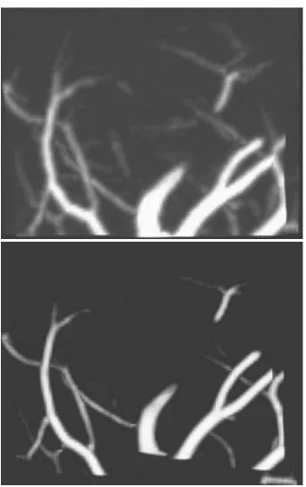
1.3 The first image is the original intensity image, the second image is the

thresh-olded vesselness measures. . . 4

1.4 An example of partial voluming effect. . . 5 1.5 An example of bifurcation, The green circled area are shared by the three

ves-sels, and its split among the three vessels is ambiguous. . . 6

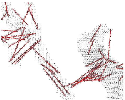
1.6 Sample results generated by random sampling approach. . . 7

1.7 Sample results generated by density based random sampling approach. . . 8

1.8 The flow diagram of our approach. The input data is a small cube (30x20x20)

cropped from the original volume. . . 9

2.1 A snapshot of vesselness orientations, most of which are along the vessels. . . . 11

2.2 Results of different steps in automatic 3D neuron tracing using all-path pruning, and this image is taken from [43]. . . 13

2.3 (a) The remaining complete reconstruction after DLP. (b) The remaining

re-construction after CLP. (c) The remaining rere-construction after an INP. . . 15

2.4 Left:Aerial image of a suburban neighborhood, Right:Graph obtained by link-ing the seed points [43]. . . 16

2.5 Left:The graph with probabilities assigned to paths using the path classification

approach. Blue and transparent denote low probabilities, red and opaque high

ones. Note that only the paths lying on roads appear in red. Right: Final reconstruction obtained by solving the Q-MIP problem [43]. . . 18

3.1 Solving line segment fitting problem in energy minimization framework. . . 21

3.2 Multi-layer graph for stereo problem, each label represents a disparity, which

is also a layer. The data points are graph nodes, the vertical arcs are data

cost(matching cost), horizon arcs are smoothness cost. . . 22

(9)

3.3 A simple min-cut problem instance. There are 9 possible s-t cuts:C ={sa,sb},{sa,bd},{sa,dt},{ac,sb},{ac,bd},{ac,dt},{ct,sb},{ct,bd},{ct,dt}. Two of the cuts{sa,bd},{sa,dt}have minimal cut costω(C)=3, which means

the min-cut solution is not unique. . . 23

3.4 An example ofα−expansionwith label cost in directed graph, from [11]. Left: s is source node and t is sink node. X1,X2..Xk are variables. y is an auxiliary

node. Right: several possible cuts on this graph. . . 26

3.5 An example ofα−expansion with label cost in undirected graph,cited from [11]. Left: each variable nodeXpis connected with sink t and auxiliary node†

at cost h/2. Right: several possible cuts on this graph. . . 27 4.1 The architecture of OpenSceneGraph. . . 28

4.2 Six slices of a small cube of the original data, these slices are cross sections.

The slice numbers are 3,13,17,23,27 and 31 from left to right and up to down.

It is hard to understand the structure of the vessels from the cross sections.. . . . 30

4.3 The 3D visualization results with MIP on the same cube, the structure is quite

clear. . . 31

4.4 Left: the 3D scene contains vesselness points and the line segments fitted to

these points. The yellow circled area shows our segment of interest. Right: the

detailed result after isolating the segment of interest, now the rotation center is

reset to this segment, notice that the rotation center has moved to this segment,

which enables us rotate and observe it more clearly. . . 32

4.5 The figure of the mechanism for object isolation. The truncated pyramid is

the perspective projection view volume, objects outside this volume will not be

rendered. The red rectangle is a the bounding box surrounding a line

segmen-t. We first build l(Pnear,Pf ar), then visit all nodes within this volume to find

the intersected objects, which should be the surrounding box of the segment

of interest. In OSG the surrounding box shares a same parent node with its

surrounded segment, so we can easily get the pointer of the segment. . . 33

4.6 Suppose the full intensity range of the data is between -4000 and 32767, and

most of the voxels have intensity range between 2000 and 6000. When we use

linear interpolation, pixels in the range between 2000 and 6000 get mapped to

a very narrow range of output intensities. If we use Window Center adjustment

(bottom image), pixels in the range from 2000 to 6000 get mapped into the full

output range. . . 34

(10)

4.7 A comparison of visualization results with and without Window Center

Ad-justment. Here we map voxels whose intensity ranges between 2000 and 6000

to the whole output range. After adjustment, the thin vessels are brighter than

before. . . 35

5.1 The flow diagram of our line segment fitting approach. . . 38

5.2 Random sampling result on a image data of size 102x96x34. There are many

segments around thick vessels, but very few segments around thin vessels. . . . 40

5.3 Sample results based on the density of vessel points. This strategy samples

less points around thick vessels and more points around thin vessels, making

the overall distribution of line segments more equal throughout the dataset.

This ensures that there is neither oversampling (leading to longer computational

time) no undersampling leading to poor model fit). . . 41

5.4 Sample result without angle agreement. . . 42

5.5 Sample result with angle agreement. . . 42

5.6 Result comparison with and without outlier model. In the first image, a wrong

segment L1 fits both inlier and one outlier point marked with ”p” in the image.

. In the second image the outlier model was added and L2 only fits the inliers.

The data cost between noise P and L2 is very high, if there is no outlier model,

L1 is definitely a better option than L2. . . 43

5.7 Line segment model. Here t is a point on the segment, x is a vessel point.

We assume that the probability of xto appear at some distance from t follows

gaussian distribution, and t is evenly distribution on the segment. So the data

cost is an infinite mixture of Gaussian distributions. . . 45

5.8 Line Model. . . 46

5.9 Result generated by line model based approach. . . 46

5.10 The Potts model, here Lp and Lqare two different labels. In our work, we set

a constant penaltyTpotts. If two points belongs to different labels the penalty is

Tpotts, otherwise the penalty is 0. . . 47

5.11 A snapshot of the Potts model result. The triangular shaped area is fitted by a

horizontal line segment , however, we want a vertical segment as neighboring

segments should have similar directions. The energy of the Potts model is

not related to the difference/similarity of line segments (labels), so it can not regularize the relative orientations of the nearby segments. . . 48

5.12 A truncated linear piecewise smoothness cost. . . 49

(11)

5.13 A 2D example of Olsson and Boykov model. Points ˜p and ˜q are noisy

mea-surements of pointspandqon the underlying curve. The quotient _||q_p−₋_qq_|02| yields

half the curvature at punder the assumption that pandqbelong to a constant

curvature segment. . . 49

5.14 Comparison results between Potts model and piece-wise smooth model. . . 50

5.15 2D example of our exhaustive grid search approach. The grid is our search

s-pace, the red line segment is the global minima, the green one is our exhaustive search result. There is some different between the two line segments, as we on-ly search points on the grid corners. But the endpoints of the global minimum

solution may be located not exactly on the grid corners. Finding a more precise

solution would require a sub-pixel search, which is too computational expensive. 51

5.16 A snapshot of fitting results based on the least squares approach. These

seg-ments are roughly correct, but their precision is not good enough, as this

ap-proach only minimizes part of the energy function in equation 5.3. . . 52

5.17 The local search approach, the green segment is the least squares solution, the

red segment is the globally optimal solution. We locally search the endpoints

within the regions surrounded by the yellow boxes. In this example, a globally

optimum solution will be found as both the endpoints of the globally optimum

solution are inside the yellow boxes. . . 53

5.18 A snapshot of fitting result based on local search. The green circle shows much

improved results compared with least squares solution in Figure 5.16. . . 54

6.1 Left: fitting result generated by line model. Right:fitting result generated by

line segment model. . . 55

6.2 A snapshot of fitting result based on the line model. As we have to ’guess’ the

length, the line segments often extend beyond what they should be. . . 56

6.3 A snapshot of fitting result based on the line segment model. . . 56

6.4 Comparison of of results with different label cost. There is no smoothness cost, and the data cost is based on the line segment model. Tv is the value of

the label cost. But there is no good value that can generates very reasonable

results. Without smoothness cost, label cost alone does not do a good job. . . . 57

6.5 Comparison of results without label cost, left (TV =0) and with the label cost,

right (Tv = 320). The smoothness cost is set to 10. The result is better with

non-zero label cost. . . 58

6.6 Fitting result without label cost, the smoothness cost is set to 30. . . 58

(12)

6.7 A snapshot of fitting result generated by Potts model, with constant label cost

and line segment model data cost. . . 59

6.8 A snapshot of fitting result generated by piece-wise smooth model. There is no label cost, the data cost is based on the line segment model. . . 60

6.9 A snapshot of fitting result generated by exhaustive grid search approach. . . . 61

6.10 A snapshot of fitting result generated by local search approach. The input of this approach is the results generated by least squares based approach. . . 61

6.11 A snapshot of fitting result generated by least squares based search approach. . 62

6.12 The left image is the input vesselness measure, the right image is the corre-spondingσestimation.σis directly proportional but not equal to the radius of the vessel. . . 63

6.13 The converged energy values ofα−expansion. . . 63

6.14 The converged energy values ofα−βswap. . . 64

6.15 A snapshot of fitting result with rings (yellow circle). . . 64

6.16 A bad case of fitting around a bifurcation. As the ambiguous area among the three vessels are not divided properly, an extra line segment is used to fit vessel voxels within the yellow circle. . . 65

(13)

List of Tables

6.1 Running times of these two approaches. . . 62

(14)

List of Appendices

(15)

Chapter 1 Introduction

1.1 Overview

Blood vessel extraction and visualization is an essential clinical task, it is essential in many

areas such as diagnosis of vascular diseases and blood flow simulation. Therefore, the

auto-mated tracing of vessel structures in 3D images has received much attention over the years

[44]. However, we have to admit that there is still a long way to go, as the medical image data

usually contains a lot of noise and the structures of vessels often exhibit complex morphology. In this thesis, we focus on automatic vessel extraction of 3D medical images.

Given an input medical volumetric image, our task is to detect the topology structure of the

blood vessels, then reconstruct and visualize those vessels. The medical volumetric images we

used are three-dimensional images that contain vessel structures. They are obtained by a CT

scanner, which is the widely used technique to create images for clinical purposes or medical science.

Our input data are micro-CT images of a mouse heart. The coronary vessels were perfused

with a radio-opaque dye called Microfil MV-122 from a company called Flowtech [1]. It is

injected in the vessels and then cures to become a solid. The mouse heart is approximately 4 mm across. Figure 1.1 shows several slices of an input medical volume, of size 585x525x892,

and these slices are cross sections. There are 892 slices in this volume but we only show

three slices, namely slices numbered 120,280 and 450. The bright regions are vessels, the

dark regions are background (muscle). In the beginning of the sequence the vessels are mainly

arteries and are pretty thick. Vessels are are getting thinner with the increase of the slice

number.

(16)

2 Chapter1. Introduction

(17)

1.2. Motivation andChallenges 3

1.2 Motivation and Challenges

A blood vessel system is just one example of a tubular tree like structure. Other examples

include neuronal arbors in optical microscopy image stacks, blood vessels in retinal scans, road

networks in aerial images, etc. Fully automated reconstruction of tubular tree like structures

remains an open computer vision problem [43].

It is very difficult to robustly deal with imaging artifacts such as noise, non-uniform illumi-nation, inhomogeneous contrasts and scene clutter. Practical systems usually require extensive

manual intervention. For example, in the DIADEM challenge [2], the algorithms with good

performance at tracing dendritic trees usually provide some good tools for manual editing. In medical science research, such editing tasks are very tedious and need prior knowledge of the

structure, which dramatically slows down the process. Recently, significant progress has been

Figure 1.2: Left: fitting result on a less curvier blood vessel. Right: fitting results on a curvier vessel.

achieved by formulating the problem as one of optimizing a global objective function [9, 45]

without any manually editing. Our work is based on a similar global energy minimization ap-proach, and is directly motivated by the graph cuts algorithm for geometric multi-model fitting

problems [10]. In particular, we model a blood vessel as a structure consisting of a sequence of

straight line segments. This is a good approximation, provided line segments are of appropriate

length. To have a good fit, for a very curved blood vessel, a shorter sequence of line segments

(18)

piecewise linear segment model and use the graph cut algorithm [7, 10] for optimization.

Figure 1.3: The first image is the original intensity image, the second image is the thresholded vesselness measures.

Before we start to fit a piecewise line-segment model to the data, we need to extract the

(19)

1.2. Motivation andChallenges 5

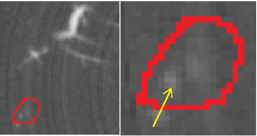
Figure 1.4: An example of partial voluming effect.

measure” [15]. A vesselness measure assigns a high value to a voxel that is likely to be a part

of a blood vessel, and a lower value to a voxel that is unlikely to be a blood vessel. Usually

vesselness measure is based on the eigenvalues of a Heissian matrix, centered at the given

voxel [15]. We threshold the vesselness measures to obtain the voxels that are likely to be

part of some vessels, and fit our piecewise line-segment model to the thresholded data. More

specifically, our labels correspond to line segments, and the task becomes to fit the thresholded

vesselness measure voxels to some line segments.

Figure 1.3 shows an original intensity image and its corresponding thresholded vesselness

measures. This data is a small cube (88x67x70) cropped from the original volume (585x525x892).

To project 3D data in 2D visualization plane, we use Maximum Intensity Projection (MIP)

technology, and we will introduce it in Chapter 4.

The Multi-model fitting approach of [19] has several advantages for our problem. First,

the energy minimization framework allows formulation of a global energy function that in-corporates any desired fitness criterion for different models, such as distance from point to a line segment, angle difference, etc. Second, by formulating the multi-model fitting problem as a optimal labeling problem, we can use existing optimization technologies, with guaranteed

optimality bounds efficiently, such asα−expansion [7] andα−βswap [7] in graph-cut. The challenges of our work mainly come from two aspects. First, there are many small

vessels that undergo partial voluming effects. A partial voluming means that part of a vessel occupies only a portion of a voxel, therefore the intensity of the partially occupied voxel is a

(20)

Figure 1.5: An example of bifurcation, The green circled area are shared by the three vessels, and its split among the three vessels is ambiguous.

which is so thin that the cross section occupies only a small portion of a voxel. Figure 1.4 is an

example of partial voluming effects. The intensity value of a partial voxel is very low due to intensity mixture, and is difficulty to be distinguished from background. However, most of the vessels are not capillaries, and are easier to segment. We want to be able to detect vessels even if they are so thin as to undergo partial voluming artifacts.

The second challenge of our approach is how to fit well around bifurcations. A bifurcation

is a place where two vessels meet and merge into one bigger vessel. It is more challenging

to accurately fit line segments at the bifurcation area, as the ambiguous area has to be divided

(21)

1.3. OurApproach 7

1.3 Our Approach

We now outline our approach in more detail. First of all, in this thesis, we assume that we

start with the thresholded vesselness measure voxels. This gives us a set of voxels that are very

likely to be vessels and we fit the piecewise line segment model to these voxels.

Next we need to fit the piecewise line segment model to the thresholded vesselness data.

A possible line segment corresponds to a distinct label in our framework. However, the space

of all possible labels is too large to handle directly. The majority of these all possible line

segments are a very poor fit for the data at hand. Following [10] , we start by sampling a set

of models, i.e. line segments that have a good chance of being a good fit. In our work we use a density based random sampling strategy. The random sampling strategy is to propose line

segments on the vessel voxels directly, this strategy provides evenly distributed segments on

vessels, and thick vessels usually get more segments than thin vessels, as shown in Figure 1.6.

Figure 1.6: Sample results generated by random sampling approach.

However, if most segments are proposed on thick vessels, there will be not enough segments

on thin vessels. So we use a density based approach to sample more segments on thin vessels

and less on thick vessels, as shown in Figure 1.7. In addition to the ”regular” line segment

models, we also need an outlier model to model outlier points, such as noise.

After sampling, we build a global energy function based on line segment model, which

consists of data cost, smoothness cost and label cost.

• The data cost measures the probability that a vessel voxel belong to a segment. It gives

(22)

Figure 1.7: Sample results generated by density based random sampling approach.

the data cost is computed as an infinite mixture of isotropic gaussian distribution on line

segment.

• The smoothness cost encourages the labeling to be consistent so that fluctuations caused

by noisy data cost are smoothed out. We also use the smoothness cost to regularize the

relative positions between neighboring segment pairs. Most of the time, two neighboring

segments on the same vessel should have similar directions, and one of their endpoints

should be close enough.

• The label cost penalizes overly-complex models, that is label cost prefers to explain the

data with fewer, cheaper models. We do not want too many line segments fitting one

vessel, so we add label cost to the energy function. For each existing model, we set a

constant penalty to control the line segment numbers.

We minimize the global energy function via a graph cut algorithm. If the smoothness term is a

metric [7] then we useα−expansionto optimize the global function, and if it is a semi-metric [7] we useα−βswap. The output of the graph cut is the optimal labeling result, which consists of several clusters. Each cluster consists of all voxels that are assigned to the same label, that

is to the same line segment. Since the set of the initial line segments may have been far from

optimal, we use these initial label results to find a possibly better set of line segment models.

Specifically, we re-estimate the line segments from the initial labeling results by re-fitting the

initial labeling with line segments of best fit. In our work, we use a local greedy search based

(23)

1.4. Outline of theThesis 9

a relatively short time. Experimental results show that these solutions give a reasonable fit in

practice.

After parameter re-estimation, we update the set of labels, that is the set of line segments

with the re-fitted models, and remove any line segment models that failed to get any support, i.e. no voxel was assigned to them. Then, we minimize the global energy function again, using

the updated set of labels. This process is iterated until the convergence of the energy, which is

guaranteed. Figure 1.8 illustrates how our approach works.

Figure 1.8: The flow diagram of our approach. The input data is a small cube (30x20x20) cropped from the original volume.

1.4 Outline of the Thesis

This thesis is organized as follows. Chapter 2 reviews and analyses the previous works on blood

vessel extraction. Chapter 3 introduces optimizing multi-labeling problem with graph cuts in

energy minimization framework. Chapter 4 introduces the 3D technology used in our work.

Chapter 5 focuses on the construction and optimization of piecewise line segment models.

Some experimental results are provided in Chapter 6. The conclusion and future work is in

(24)

Chapter 2 Related Work

Extracting curvilinear structures automatically and robustly is of fundamental relevance to many scientific disciplines, especially in medical research, such as fine modeling of complex

blood vessel structures, automated delineation of linear structures in aerial imagery

databas-es. Recently, there has been a resurgence of interest in automated delineation techniques

[13, 24, 32, 34], which can be categorized into greedy strategies methods [26, 40] and

graph-based methods [14, 37, 43, 45, 50]. In this chapter, we will briefly review several related

methods for automatical delineation of linear structures that form complex and potentially

loopy networks.

2.1 Greedy Strategies and the Vesselness Measures

Greedy strategies start from a set of seed points, incrementally grow branches by evaluating a local tubularity measure usually based on the Hessian and Oriented Flux matrices [26, 40].

High tubularity paths are then iteratively added to the solution and their end points are treated

as the new seeds from which the process can be restarted. Since the search typically involves

processing only a part of the image data, these methods are computationally fast. However,

they lack robustness to large gaps in the image data as they are sensitive to imaging artifacts

and noise.

In our work, we use tubularity vesselness measure as the input data. A vesselness measure

is obtained on the basis of all eigenvalues of the Hessian. Letλ1,λ2andλ3be the eigenvalue of

the Hessian (|λ1| ≤ |λ2| ≤ |λ3|). For a point belongs to an ideal tubular structure in a 3D image,

λ1should be pretty small (ideally zero), andλ2andλ3should be of a large magnitude and equal

(25)

2.1. GreedyStrategies and theVesselnessMeasures 11

sign. The sign is an indicator of brightness.

|λ₁| ≈0|

|λ₁| |λ₂|

λ2≈ λ3

(2.1)

The respective eigenvectorsu1,u2,u3point out singular directions:u1indicates the direction

along the vessel, which is also the minimum intensity variation. We use u1 as the vesselness

orientation. u2 andu3 form a base for plane orthogonal to u1. Figure 2.1 is a snapshot of a

vesselness orientation result. In medical images, vessels emerge as bright tubular structures in

a darker environment. This prior information can be used as a consistency check to discard

structures present in the image with a polarity different than the one sought. The vesselness

(26)

12 Chapter2. RelatedWork

measure function is defined as:

f(x)=

          

0 λ2 >0 orλ3> 0

1−exp

−R2A

2α2

exp

−R2B

2β2

1−exp−S2

2c2

otherwise (2.2)

whereRAandRBare two geometric ratios based on the second order ellipsoid,S is the second

order structureness measure. α,βandcare thresholds which control the sensitivity of the line filter to the measures RA, RB and S. RA =

|λ2|

|λ3| refers to the largest area cross section of the

ellipsoid and accounts for the aspect ratio of the two largest second order derivatives. It is

essential for distinguishing between plate-like and line-like structures, since only in the latter

case it is zero. RB =

|λ1|

√

|λ2λ3| accounts for the deviation from a blob-like structure but cannot

distinguish between a line-like and a plate-like pattern; it attains its maximum for a blob-like

structure and is zero whenever λ1 ≈ 0, orλ1 andλ2 tend to vanish. S = q

P

j≤3λ2j will be a

low value in the background where no structure is present and the eigenvalues are small for the lack of contrast. In regions with high contrast compared to the background,S should be a

larger value since at least one of the eigenvalues will be large.

2.2 Graph-based Methods

Graph-based methods find seed points in the whole image or volume by evaluating the

tubular-ity measure [14, 37] densely and finding its local maxima [14, 37, 43, 45, 50]. Although this

is more computationally demanding, it can still be done efficiently in Fourier space or using GPUs [12, 26, 27]. The seed points are then connected by paths that follow local maxima of

the tubularity measure. This results in a graph that forms an overcomplete representation of

the underlying tree structure and the final step is to build a tree by selecting an optimal subset

of the edges. This can be done by finding the Shortest Path Tree (SPT) [37], the Minimum Spanning Tree (MST) [14, 53], the k-Minimum Spanning Tree (k-MST) [45], or a solution to

the Minimum Arborescence Problem (MAP) [43]. Some graph-based methods are introduced

in this section.

2.2.1 Automatic 3D neuron tracing using all-path pruning

The reconstruction of a neuron is defined as a set of topologically connected structure

com-ponents that describe the 3D spatial morphology of this neuron in a 3D image. This

neuron-tracing method consists of two major steps, in the first step an initial over-complete

(27)

2.2. Graph-basedMethods 13

are pruned. SC is a loosely defined concept that could mean neuron branches, individual

re-construction node,voxels or other sub-structures contained in the neuron rere-construction. Figure

2.2 shows the results of different steps in this paper.

Figure 2.2: Results of different steps in automatic 3D neuron tracing using all-path pruning, and this image is taken from [43].

Initial Reconstruction

The input of this method is a 3D neuron image I and a seed Ps(xs,ys,zs) that is within the

neuron region. Ps is often a bright spot of the neuron and can be automatically detected. A

global thresholdta is used to define the image foreground, that is, any voxel that has smaller

value than ta is assumed to be background, otherwise it belongs to foreground. Typically ta

is set to be the average intensity value of the entire image. After the global thresholding, a

median filter is applied to remove noise.

(28)

geodesic metric function which is define as:

e(v0,v1)= ||vo−v1|| gI(vo)+gI(v1) 2

!

gI(p)=exp

λI(1−I(p)/Imax)2

,

(2.3)

v0 = (x0,y0,z0) and v1 = (x1,y1,z1) are two adjacent foreground voxels, and their spatial coordinates must satisfy|x0−x1| ≤ 1,|y0−y1| ≤ 1,|z0−z1| ≤ 1. As G only contains edges of adjacent voxel-vertices, it is highly sparse. I(p) is the intensity value for voxel p,Imaxis the

maximum intensity of the entire image I.λIis a positive coefficient.

Then Dijkstra algorithm is applied to G to find the shortest paths from the seed Ps to all

other vertexes in G. In the resultant shortest path map, the vertices that have no child are leaves.

Obviously, a path can be traced back from every leaf vertex to the seed Ps, which is the root

vertex. All these paths share many common sub-paths. The entire solution can be organized as

a tree graphGT. Since it contains all ordered paths from the root to all foreground voxels, the

building of this tree graph is called the all-path reconstruction, and it is an ICR.

Pruning a reconstruction

Since the ICR contains all the possible paths and thus could contain redundant SC, the

redun-dant structural elements need to be pruned by a maximal covering minimal-redunredun-dant (MCMR)

subgraph algorithm. MCMR consists three pruning steps: Dark-leaf pruning (DLP),Covered-leaf pruning (CLP) and Inter-node pruning (INP).

DLP removes dark leaf nodes from GT. In the beginning, the input image is

threshold-ed by ta. ta is a very low value so that all possible paths in the neuron can be captured and

any potential connectivity of any possible neuron regions connecting to the seed can be

maxi-mized. However,tais so low that the foreground often contains many dark voxels. In an ICR,

these dark voxels correspond to many redundant branches. The DLP iteratively removes the leaf nodes whose intensity value is lower thantv. tv is a new threshold that defines the lowest

bright voxel intensity. After DLP, the structure complexity is reduced, while the connectivity

of different regions is still maximized. In CLP, a radius-adjustable sphere centered at a recon-struction node is defined, the radius gradually increases until 0.1% of the image voxels within

this sphere that are darker than ta. Each of the reconstruction nodes, along with its estimated

radius are treated together as an SC. For two SCs,aandb, a is significantly covered bybif the

following condition is satisfied:

(29)

Figure 2.3: (a) The remaining complete reconstruction after DLP. (b) The remaining recon-struction after CLP. (c) The remaining reconrecon-struction after an INP.

Ω(.) computes the volume of the occupied region of a reconstruction node. This equation tells us whether nodebis significantly covered by node a. When a leaf node is covered by another

node or several other nodes jointly,this leaf node should be pruned, otherwise the leaf node should be kept. CLP checks all the leaf nodes and removes those being significantly covered

by other nodes. This pruning process is iterated until no more leaf node can be pruned.

After CLP, all neuron regions have been reached by a minimum number of leaf nodes. Then

INP is applied to remove the redundant inter-nodes that connect leaf nodes to branch nodes or

(30)

branching node or the root and is significantly covered bya, then b is pruned and a0sparent

is updated asb0soriginal parent. Ifbis not pruned, then a same check should be executed on

bsnon-branching-node parent. For each node, this process is iterated until a branching parent

node or the root is reached.

2.2.2 Automated Reconstruction using Path Classifiers and Mixed

Inte-ger Programming

In this approach, first a directed graph is constructed, which is an over-complete representation

for the underlying network of tubular structures. Then a Q-MIP (Quadratic Mixed Integer

Programming) problem is formulated to find the most likely arborescence. As well, a path classifier is trained to provide probabilistic weights, which are of great importance to Q-MIP.

Graph Construction

Figure 2.4: Left:Aerial image of a suburban neighborhood, Right:Graph obtained by linking the seed points [43].

There are three steps to build a directed graph G. First, a scale space tubularity measure

based on the oriented flux cross-section trace measure [26] is computed. This measure is used

to assess if a voxel lies on a centerline of a tubular at a given scale. Second, seed points are

sampled from the input image by iteratively selecting the maximum tubularity points and then

suppressing their neighboring points. Finally, paths linking the seed points are computed using

(31)

Q-MIP Formulation

After constructing a directed graph G, this problem is solved by minimizing the following

energy equation

arg min

t∈T(G) X

ei jk∈F

ci jkti jk (2.5)

where t is the arborescence in G; T(G) is the set of all possible arborescence. F = {ei jk =

(ei j,ejk)} is the set of pairs of consecutive edges in G, ei jk = (ei j,ejk) represents a pair of

consecutive edges ei j and ejk, ei j = (vi,vj) is the geodesic tubular path linking seed points

vi,vj. ci jk encodes the geometric compatibility of consecutive edges ei jk, and ti jk denotes the

presence or absence ofei jk in the arborescence. The geometric compatibilityci jkis defined as

the probability likelihood ratios assigned to edge-pairs:

ci jk= −log        

PTi jk= 1|Ii jk,pi jk

PTi jk= 0|Ii jk,pi jk         (2.6)

whereIi jkrepresents image data around the tubular path pi jk, the probabilityP(Ti jk= 1|Ii jk,pi jk)

denotes the likelihood of the path pi jkbelonging to the arborescence, which is computed based

on global appearance and geometry of the paths.

By decomposing the indicator variableti jkas the product of the two variablesti jandtjk, the

minimization of the energy function can be formulated as the Q-MIP:

arg min

t∈T(G) X

ei j,ejk∈E

ci jkti jtjk (2.7)

This Q-MIP problem is NP-Hard, its solution can be found up to an arbitrarily small tolerance

from the true optimum using a branch-and-cut strategy [43].

Path Classification

The results of the Q-MIP optimization depends heavily on the probabilistic weights ci jk. A

standard approach to computing such weights is to integrate tubularity values along the

path-s. However, this approach is often unreliable because a few very high values along the path might offset low values, and fail to adequately penalize spurious branches and short-cuts. Fur-thermore, it is often difficult to balance between allowing paths to deviate from a straight line and preventing them from meandering too much. The path-classification approach computes

the probability estimates using a more reliable way. First, a tubular path is broke down into

several segments and one feature vector is computed based on gradient histograms for each

(32)

Figure 2.5: Left:The graph with probabilities assigned to paths using the path classification approach. Blue and transparent denote low probabilities, red and opaque high ones. Note that only the paths lying on roads appear in red. Right: Final reconstruction obtained by solving the Q-MIP problem [43].

mappings. The path is divided into equal-length overlapping segments, and for each segment

the histogram is computed for points belonging to a certain neighborhood around the centerline with a certain radius.

Then an embedding approach is used to compute fixed-size descriptors from the potentially

arbitrary number of feature vectors. To derive from them a fixed-size descriptor, a

Bow(Bag-of-Words) approach is used to compactly represent the feature space. The words of the BoW

model are generated by randomly sampling a predefined number of descriptors from the

train-ing data. For a given path of arbitrary length, the embeddtrain-ing of the HGD descriptors are

computed into the codewords of the model. Adapting the sequence embedding approach of

[51], the minimum Euclidean distance is calculated from the paths descriptors to each word in

the model. This yields a feature vector of minimal distances that has the same length as the number of elements in the BoW model.

Finally, the descriptors are feed to a SVM classifier to compute a probability estimate.

To train the SVM classifier, the positive and negative paths are randomly sampled from the

ground-truth trees associated to the training images. To obtain negative samples, the tubular

graphs are first built in these training images, then paths are randomly selected from these

graphs and matching paths are found in the ground truth tree. For a given path, this is done by

finding the two nodes of the tree that are closest to the start and end points of the path.

(33)

but cross the background. Thus, it discourages shortcuts, which is something that integrating

(34)

Chapter 3 Energy Minimization Framework

The energy minimization framework is popular for a variety of computer vision applications.

There are mainly two steps in the energy minimization framework. First, build an energy

function, then optimize the energy function. Usually it is difficult to design an appropriate energy function, and optimizing the function is also not an easy task. However, it is still a

popular framework for several reasons. Firstly, this is a common framework which standard

optimization methods can be applied to once the energy function is built. Also one can easily

incorporate various prior knowledge into the energy function. Besides, the value of the energy

function provides an effective way to evaluate the solution and can be used as a guide in the optimization algorithm [31].

Many of the important developments in computer vision began with a proposal for a better

energy, a better algorithm for an energy, or a combination of both [11]. Researchers try to use

algorithms that are both effective in theory and fast in practice to optimize new energies. Graph cut is an optimization algorithm in the energy minimization framework that has been widely

used in a variety of vision problems [46], including stereo and motion [3, 6, 7, 30, 38, 39, 20,

22], image segmentation [5], image restoration [6, 7, 18, 21], image synthesis [25],

multi-camera scene reconstruction [41], and medical imaging [4, 8, 23]. The output result generated

by a graph cut algorithm is often a global minima, while in some case [6, 18, 21, 30], it is local

minima, but still within a known factor of the global minima [7].

Our algorithm implements multi line segment fitting based on a graph-cut algorithm, which works in the energy minimization framework. The task of line segment fitting is posed as a

multi labeling problem, which can be solved by minimizing an energy function. The

max-flow/min-cut algorithm can globally optimize the energy function. The way to solve multi-model fitting problem in the framework of energy minimization is shown in Figure 3.1.

In this chapter we will first introduce the way to solve line segment fitting problem in the

framework of energy minimization in Section 3.1, then review several well-known concepts on

(35)

3.1. FromMultiLineSegmentFitting toLabelingProblem 21

which subsequent chapters are based. Section 3.2 explains the s-t min-cut problem. Section 3.3

explains the move-making algorithms “α-expansion” and “αβ-swap” for optimizing the multi-label energies [7]. We use these move-making algorithms to optimize our energy function.

Figure 3.1: Solving line segment fitting problem in energy minimization framework.

3.1 From Multi Line Segment Fitting to Labeling Problem

Traditionally, to get trajectory of a 3D vessel inside 3D medical images, the clinician must

manually define some points on the path using 3D orthogonal views. But for a complex

struc-ture this path construction task becomes very tedious and one can easily made mistakes. The

goal of our work is to get the topology of the 3D vessel structure in a automatic way.

Our approach uses multiple line segments to fit blood vessels, which is a geometric

multi-model fitting problem. Geometric multi-multi-model fitting is a typical chicken-egg problem: data

points should be clustered based on geometric proximity to models whose unknown parameters must be estimated at the same time [19]. Currently, most existing methods such as RANSAC

[42, 47, 54], ignore the overall classification of all points, and just greedily search for models

with most inliers that are within a threshold. In this paper we formulate the multi-model fitting

problem as an labeling problem, each geometric model is treated as a label, and a global energy

function is built to balance the regularity of inlier clusters and geometric errors.

A labeling problem is the task of assigning an explanatory label to each element in a set

(36)

22 Chapter3. EnergyMinimizationFramework

each label represent a cluster of points, and each point could be assigned to a label. Clearly,

we can treat the task of multi-model fitting problem as a labeling problem.

To describe a labeling problem, one needs a set of data points and a set of labels. A

discrete labeling problem associates one discrete variable with each data point, and the goal of optimization is to find the best labeling to these variables, which must satisfy some global

energy constraints. In computer vision, the data points can be things like pixels in 2D images

or voxels in 3D image, disparity measurement in stereo matching, and intensity measurements

from CT/MRI. The labels are typically either semantic (car, pedestrian, street) or related to the scene geometry (depth, orientation, shape, texture) [10]. Figure 3.2 shows an example of

transforming stereo matching to a multi-label problem.

Figure 3.2: Multi-layer graph for stereo problem, each label represents a disparity, which is also a layer. The data points are graph nodes, the vertical arcs are data cost(matching cost), horizon arcs are smoothness cost.

Assume set P contains all data points,ζcontains all labels. We associate a discrete variable with each p ∈ P, and each variable p is allowed to take one label from set ζ. The goal of discrete labeling is to complete a map f:P7→ ζwhich assigns a label fpto each element p ∈P.

In geometric model fitting, the map f assigns labels fp to 3d image voxels. In this thesis, we

(37)

3.2. The s-t min-cut problem 23

3.2 The s-t min-cut problem

To define an s−tmin-cut problem, we need a directed graphG=(V,A), and two designated terminals s,t ∈ V, s is source node and t is sink node, an arc cost ω(u,v) ≥ 0 for each (u,v)∈ A. Thes−tmin-cutC=(S,T) is a partition ofVinto two disjoint setsS andT such that s ∈ Sand t ∈ T. The cut-set ofCis the set{(u,v) ∈ A|u ∈ S,v ∈ T }. The goal of s-t min-cut is to find and remove the cheapest cut-set C so that there is no path from s to t. The

cost of this cutω(C) is the total cost of all arcs in C.

Figure 3.3 shows an instance of the min-cut problem. The capacity of an edge is a mapping

Figure 3.3: A simple min-cut problem instance. There are 9 possible s-t cuts: C = {sa,sb},{sa,bd},{sa,dt},{ac,sb},{ac,bd},{ac,dt},{ct,sb},{ct,bd},{ct,dt}. Two of the cuts {sa,bd},{sa,dt} have minimal cut cost ω(C) = 3, which means the min-cut solution is not unique.

c : A → R₊, denoted bycuv. It represents the maximum amount of flow that can pass through

this edge. A flow of an edge is a mapping f :A→R₊, denote by fuv. There are two constrains

with a flow: the flow fuv can not exceed its capacity cuv, and the sum of the flows leaving a

node must equal with the sum of flows entering this node, except for the sink node and source

node. The value of flow is defined by|f| = P

u∈v fsv, where s is the source node. It represents

the amount of flow passing from the source to the sink. The maximum flow problem is to

maximize|f|, and the maximum value of an s-t flow is equal to the minimum capacity over all

s−tcuts [36]. In optimization theory, max-flow/min-cut theorem is stated as follows:

Theorem 3.2.1 A. f is a maximum flow.

B. there exists an s-t cut which capacity is equal to the value of f.

(38)

Max-flow/min-cut theorem implies that in a flow network, the min-cut can be computed in a low order polynomial time by a number of classical s− t maximum flow algorithms [31].

Cormen et al. in [28] describe an augmenting path strategy to compute the minimum cut of a

graph. Goldberg and Tarjan [17] proposed an push-relabel approach to solve the minimum cut problem.

3.3 Multi-Label Energy Minimization

The multi-label energy implies that the label set has cardinality|L|> 2. Thes−tcut reduction is inherently fit for two label problems because there are two terminalssandt. There are special

local search algorithms for direct energy minimization, also called move-making algorithms in the computer vision literature [11]. We will explain two move making algorithms in that use

graph cuts: the “α-expansion” algorithm and “αβ-swap” algorithm. The two algorithms find approximate solutions by decreasing the energy on appropriate graphs iteratively, which leads

to significantly better solutions than the previous algorithms based on ‘standard’ moves. In our

experiment we use both “α-expansion” algorithm and “αβ-swap” algorithm.

3.3.1 “

α

-expansion”

The α-expansion algorithm performs local search on multi-label energies. Given current la-beling f, the idea of oneα-expansion move is as follows: all variables should either switch to a particular labelαor keep its current label. For a particular labelαthere are an exponential number of possible moves. Intuitively,α- expansion means the labelαcan expand its region. Theα-expansion algorithm is implemented as shown as below.

1. start with an arbitrary labeling f

2. while true

3. for each labelα∈ L

4. Find ft=argminE(f) among ft within one ”α-expansion” move of f

5. if E(ft)<E(f)

6. f=ft

7. if converged

8. return f

(39)

3.4. LabelCost inGraphCut 25

with metric interaction penalty V. V is called a metric on the space of labelsLif it satisfies

V(α, β)=0⇔ α= β V(α, β)=V(β, α)≥ 0 V(α, β)≤V(α, γ)+V(γ, β)

(3.1)

where labelsα, β, γ∈ L.

3.3.2 “

αβ

-swap”

Theαβ-swap algorithm performs local search using a different kind of moves. Given a current labeling f, the idea of oneαβ-swap move is as follows: all variables with fp ∈ {α, β}choose

a new label inα, β. That is each variable with label fp ∈ {α, β}could either swap to the other

label or just keep its current label. Theαβ-swap algorithm is implemented as shown as below.

1. start with an arbitrary labeling f

2. while true

3. for each pair of labelsα, β∈ L

4. Find ft=argminE(f) among ft within one ”αβ-swap” move of f

5. if E(ft)<E(f)

6. f=ft

7. if converged

8. return f

Theαβ-swap algorithm could be used to approximately minimize the energyE(f) with semi-metric interaction penalty V. V is called a semisemi-metric on the space of labelsLif it satisfies

V(α, β)= 0⇔ α= β V(α, β)=V(β, α)≥ 0

(3.2)

3.4 Label Cost in Graph Cut

In a basic energy E(f) = P

pDp(fp), the optimal fp can be computed by minimizing data

cost independently. However, we might want to use as few unique labels as necessary. For

example, in model fitting we do not want to use too many models, we prefer to fit the data

points with fewer models. Then we can introduce a new energy term, which balances the

(40)

unique models. This new energy term is called as label cost and it penalizes each existing

unique label in f.

E(f)= X

p∈P

Dp(fp)+ X

l∈L

H(l)·δl(f) (3.3)

Elabelcost = X

l∈L

H(l)·δl(f) (3.4)

whereH(l) is the non-negative label cost of label l,δl(f) is the indicator function

δl(f)=         

1 ∃p: fp =l

0 otherwise

(3.5)

The label cost can be viewed as a special case of global interactions recently studied in com-puter vision by Werner [16] and Woodford [19]. Werner proposed a cutting plane algorithm to

make certain high-order potentials tractable in an LP relaxation framework [16]. However, this

algorithm is very slow. In [10] they proposed a fast algorithm to minimize energy with label

cost, by extending theα−expansionalgorithm to incorporated label cost at each expansion. Figure 3.4 and 3.5 showsα−expansionwith label cost in both directed and undirected graph for labelβ.

Figure 3.4: An example ofα−expansionwith label cost in directed graph, from [11]. Left: s is source node and t is sink node.X1,X2..Xkare variables.yis an auxiliary node. Right: several

possible cuts on this graph.

In Figure 3.4, an auxiliary nodeyis introduced to construct a subgraph. The cost between each variable node Xp to auxiliary node y is h. y is connected with sink node t. The cost

betweenyand node t is h, which means the max-flow of this subgraph could not exceed h. So

in a minimal s-t cut, the subgraph contributes cost is 0 if noXpis assigned to labelβ(cut 1), as

there is no cut on this subgraph. Otherwise it is h (cut 2,4,5), in such case there is at least one

Xp is assigned to labelβ. Cut 3 could not be a min-cut as its cost is greater than h.

(41)

3.4. LabelCost inGraphCut 27

Figure 3.5: An example ofα−expansionwith label cost in undirected graph,cited from [11]. Left: each variable node Xp is connected with sink t and auxiliary node† at cost h/2. Right:

several possible cuts on this graph.

the min-cut value of this subgraph is 0 (cut 1). If at least one node is assigned labelβ, then the the subgraph contributes cost h (cut 3,cut 4). Cut 2 could not be a min-cut with respect to

(42)

Chapter 4 3D Visualization

The 3D visualization plays a very important role in our work, that is visualization of the input

3D volumes and output results. As well, we also need to develop some assistant tools to help

us to evaluate and debug the results of model fitting in a convenient setting. In this chapter, we

introduce our development platform and relevant technologies that are used in our work.

4.1 3D Development Platform

Figure 4.1: The architecture of OpenSceneGraph.

(43)

4.2. MaximumIntensityProjection 29

We develop our 3D programs based on OSG (OpenSceneGraph) [33], which is an open

source 3D graphics application programming interface. It is entirely based on OpenGL [52],

which ensures it to be a multi-platform application programming interface for drawing 3D and

2D graphics. But it goes beyond OpenGL by providing common function to many 3D appli-cations, such as texture mapping, level of detail control, 3D file and image loaders. Because

of its rich features and open source license, OSG has been used by application developers in

fields such as visual simulation, virtual reality, scientific visualization and computer games.

Besides, OSG is written in Standard C++language, using the standard template library (STL) for containers, which makes it quite compatible with our main program.

OSG is a well-designed rendering middleware application, which is actually a deferred

rendering system based on the theory of a scene graph. A deferred rendering system records

rendering commands and rendering data in a buffer so that the commands can be executed at a later time. This deferred rendering design allows the system to perform various optimizations

before rendering, as well as implement a multi-threaded strategy for handling complex scenes.

A scene graph is a general data structure which represents the 3D worlds as a graph of nodes

that contain logical and spatial relationship information.

Typically a scene graph is represented as a hierarchical graph, which contains a set of nodes.

Usually there is a top root node, several group nodes which can contain any number of child

nodes. There are also a number of leaf nodes, which serves as the bottom layer of the graph.

A group node can have an unlimited number of child nodes, and child nodes that belong to

the same group node can be treated as one unit and share the information of the parent node.

An operation performed on a parent node will be propagated to all the child nodes by default.

A typical scene graph tree does not allow isolated elements and directed cycles. Sometimes a child node may have more than one parent node, which means this node is considered to be

”instanced”, and the scene graph can be defined as a directed acyclic graph (DAG). Instancing

produces many interesting effects, including data sharing and multi-pass rendering [49].

4.2 Maximum Intensity Projection

The maximum intensity projection (MIP) is a volume rendering method for 3D data that projects in the visualization plane the voxels with maximum intensity that fall in the way of

parallel rays traced from the viewpoint to the plane of projection [48]. If using orthographic

projection, then two MIP renderings from opposite viewpoints will be symmetrical images. In

OSG it is quite convenient to use MIP, first we need to build a 3D texture for the input volume

and sent it to the scene graph, then we set the rendering option to be MIP MODE and render a

(44)

30 Chapter4. 3D Visualization

(45)

4.3. Isolating3D Objects ofInterest 31

Figure 4.3: The 3D visualization results with MIP on the same cube, the structure is quite clear.

selecting the points with maximum intensity.

Figure 4.2 shows several slices of an input data cube, of size 102x96x34, and these slices

are cross sections. There are 34 slices and we show six of them, namely slices numbered

3,13,17,23,27 and 31. From these slides, it’s impossible to figure out the structure of the

vessels, but from the MIP projection, the structure becomes clear, which is illustrated in Figure

4.3.

However, the 2D MIP projection looses depth information, and cannot provide complete

information about the original 3D data. To improve the sense of 3D, in our program we allow

to rotate the 3D data, during the rotation we continue rendering the new MIP results under a different view. This way, the users can perceive the relative 3D positions of the data compo-nents. So we use the orthogonal projection, no adjustment for distance from the camera made

in this projection, so that objects on the screen will appear the same size no matter how close

or far away they are. There are also some drawbacks in orthogonal projection, it is difficult for user to distinguish between left and right, front and back. However, as we can rotate to a

(46)

Figure 4.4: Left: the 3D scene contains vesselness points and the line segments fitted to these points. The yellow circled area shows our segment of interest. Right: the detailed result after isolating the segment of interest, now the rotation center is reset to this segment, notice that the rotation center has moved to this segment, which enables us rotate and observe it more clearly.

4.3 Isolating 3D Objects of Interest

Beside 3D visualization, we also need some assistant tools for visualizing and debugging the

model fitting results. For example, if we want to know how well a specific segment fits the

vessels points that are assigned to it, we need to rotate this segment to an appropriate angle,

and zoom it into a proper scale, so that we can observe the fitting details more clearly. If we try

to perform this test on the full model, this is cumbersome for the user and also computationally

inefficient, especially when there are many segments in the results. Usually, there will be more than 200 line segments for fitting a medium data set (200*120*100), and a lot of segments

overlap with each other. The overlap makes it more difficult to observe the fitting quality, even after careful rotation and zooming in.

So we developed a 3D segment isolation tool to solve this problem. The isolation tool is

quite easy to use, the user just need to double click the segment of interest, then other segments

will be hidden from the view and the chosen segment will be displayed on the screen alone,

together with the vessel points assigned to it. If the user double click this segment again, then

(47)

4.3. Isolating3D Objects ofInterest 33

Figure 4.5: The figure of the mechanism for object isolation. The truncated pyramid is the perspective projection view volume, objects outside this volume will not be rendered. The red rectangle is a the bounding box surrounding a line segment. We first build l(Pnear,Pf ar),

then visit all nodes within this volume to find the intersected objects, which should be the surrounding box of the segment of interest. In OSG the surrounding box shares a same parent node with its surrounded segment, so we can easily get the pointer of the segment.

tool.

To implement the isolation tool, we need to transform the coordinates of the clicked points.

There are two important coordinate systems in OSG, the world coordinates and the screen

co-ordinates. The world coordinate system is also known as the universe coordinate system. This

is the base reference system for the overall model in 3D, to which all other model coordinates

relate. The screen coordinate system refers to the physical coordinates of the pixels on the

computer screen, based on current screen resolution. When clicking on the screen, we can get

the mouse position x and y. Let the point Pm(x,y) belong to screen coordinate system. We

need to convert it to a pointPwin world coordinate system. To perform the transformation, we

need to use a series of matrices, such as projection matrix and model view matrix, which are provided in the public interfaces of OSG.

In Figure 4.5, we build a ray that starts from the project reference point and passes through

Pm. Its intersection point with the Front Plane is pnear, the intersection point with the Back

Plane is pf ar. We can calculate pnear and pf ar by back projection with the projection matrices.

The world coordinate point Pw is located on the line segment l(pnear,pf ar). We visit all the

(48)

OSG due to its scene graph structure, we only need to visit nodes in the view volume, not all

scene graph.

To isolate a segment, the user need to click right on it. This is quite a tough task as the

segments are too ‘thin’ to be clicked on easily. To solve this problem, we add a hidden bounding box for each line segment. Each box is added to the direct parent node of its corresponding

segment. If the box is clicked, we can easily find out its corresponding segment as they share

the same parent in the scene graph. The surrounding boxes are set to be invisible, so that the

user is not distracted by them.

4.4 Window Center Adjustment

Figure 4.6: Suppose the full intensity range of the data is between -4000 and 32767, and most of the voxels have intensity range between 2000 and 6000. When we use linear interpolation, pixels in the range between 2000 and 6000 get mapped to a very narrow range of output inten-sities. If we use Window Center adjustment (bottom image), pixels in the range from 2000 to 6000 get mapped into the full output range.

The intensity of each voxel in the original 3D image ranges from -4000 to 32767. However,

(49)

4.4. WindowCenterAdjustment 35

Figure 4.7: A comparison of visualization results with and without Window Center Adjust-ment. Here we map voxels whose intensity ranges between 2000 and 6000 to the whole output range. After adjustment, the thin vessels are brighter than before.

output gray level, therefore, when we map the output gray range to the input gray range, we

are likely to loose a lot of important details, as shown in Figure 4.6. Most voxels have intensity

in the range from 2000 to 6000, but after mapping them to a narrow range of intensities, lots of important details were lost.

We use a window center adjustment approach to solve this problem. We set a window on

(50)

exceed the interest range size. Then we map the input gray level within the window to 0-255,

according to Equation 4.1.

f(I)=

                

0 I < Ic−W/2

255 I > Ic+W/2

(I−Ic+W/2)·(255/W) otherwise

. (4.1)

whereIcis the center of the window,Wis the window size, I is the input intensity value. With

window-center approach, we can assign our input range of interest to the largest possible output

Automatic Multi-Model Fitting for Blood Vessel Extraction

Scholarship@Western

Scholarship@Western

Automatic Multi-Model Fitting for Blood Vessel Extraction

Automatic Multi-Model Fitting for Blood Vessel Extraction

AUTOMATIC MULTI-MODEL FITTING FOR BLOOD VESSEL

EXTRACTION

(Thesis format: Monograph)

by

Xuefeng Chang

Graduate Program in Computer Science

A thesis submitted in partial fulfillment

of the requirements for the degree of

Masters of Science

The School of Graduate and Postdoctoral Studies

The University of Western Ontario

London, Ontario, Canada

c

Abstract

Acknowledgements

Contents

List of Figures

List of Tables

List of Appendices

Chapter 1

Introduction

1.1

Overview

1.2

Motivation and Challenges

1.3

Our Approach

1.4

Outline of the Thesis

Chapter 2

Related Work

2.1

Greedy Strategies and the Vesselness Measures

2.2

Graph-based Methods

2.2.1

Automatic 3D neuron tracing using all-path pruning

2.2.2

Automated Reconstruction using Path Classifiers and Mixed

Inte-ger Programming

Chapter 3

Energy Minimization Framework

3.1

From Multi Line Segment Fitting to Labeling Problem

3.2

The s-t min-cut problem

3.3

Multi-Label Energy Minimization

3.3.1

“

α

-expansion”

3.3.2

“

αβ

-swap”

3.4

Label Cost in Graph Cut

Chapter 4

3D Visualization

4.1

3D Development Platform

4.2

Maximum Intensity Projection

4.3

Isolating 3D Objects of Interest

4.4

Window Center Adjustment