EFFECTIVE CLASSIFICATION BASED ON CORRELATION ANALYSIS

(1)

481 | P a g e

EFFECTIVE CLASSIFICATION BASED ON

CORRELATION ANALYSIS

Himani Chauhan, Garima Saxena, Arpit Tripathi,

Computer Science, Galgotia’s College of Engineering & Technology, India

ABSTRACT

This work deals with the problem of fashioning a fast and accurate data classification, learning it from a

possibly small set of information that might be already categorized. The proposed method is primarily based on

the framework of the so-called Logical Analysis of Data (LAD), but enriched with facts received from statistical

considerations on the records. The accuracy of the proposed approach is compared to that of the usual LAD

algorithm, on publicly available datasets of the UCI repository.

Index Terms: Classification Algorithms, Data Mining, Discrete Mathematics, Machine Learning,

Optimization

I. INTRODUCTION

Logical analysis of data (LAD) is a mathematical methodology which comprises ideas and concepts from optimization, combinatories and Boolean functions.[1] [2] [3] The fundamental concept in LAD is that of

patterns, or rules, which were found to play a decisive role in classification, clustering, detection of subclasses, feature selection, medical diagnosis, marketing and other problems.

The research area of LAD was initiated by Peter L. Hammer in 1986, who helped the methodology to be successful in many data analysis applications. Although LAD has been used in many data analysis applications but one of the predominant goals of LAD is to classify new observations with prior knowledge of supervised data sets[]. The available information consists of a set of observations with a class label assigned to them. The LAD aims at detecting logical patterns from training set, which distinguish observations in one class from all the other observations. Different approaches have been proposed including Neural Networks, Support Vector Machines, K-Nearest Neighbours Bayesian approaches, Decision Trees.[2][4]

This overview presents some of the basic characteristics of LAD, from the description of the main ideas to the implementation of effective algorithms for pattern generation and proposes an original enhancement to this methodology based on statisticalconsiderations on the data. Originally, it was used to analyze binaryattributes only but it turned out later that most of the real-life applications include attributes taking real values, so a “binarization” method was proposed.[1] Binary attributes, generated using specific values called “cut-points”, constitutes a support which are combined for generating logical rules called patterns. These patterns are used to classify each unclassified record.

(2)

482 | P a g e

with result, result being the attribute specifying the class label to which the observation belong. Correlation between two attributes is defined as the linear relationship between two attributes, i.e. how two attributes are related with each other, what form of relationship they comply with. Correlation between attributes is measured as correlation coefficient, which may be positive as well as negative. If correlation coefficient of two attributes is close to +1 or -1, this means both these attributes are linearly dependent. For a pair of independent attributes, correlation coefficient is zero but the converse is not true as correlation coefficient is the measure of linear dependence so if two attributes have zero correlation coefficient, then either they are independent or they are not linearly dependent.

II. NOTATION AND TERMINOLOGY

The classifier is trained using a set of past observations denoted by S. Each observation of set S is mapped to a label, specifying the class it belongs to. The training set S is partitioned into two subsets S+ and S- representing the positive and the negative observations, respectively. The overall performance of the trained classifier is evaluated using a test data set T. The comparison of the predicted classification (given by the learned classifier) of T to its real classification results to the classification errors of our classifier.

An archive (S+, S-) of the type described above can be naturally represented by a partially defined Boolean function i.e., a mapping S→ {0, 1}, where S is viewed as a subset of {0, 1}n_{. Any completely defined Boolean}

function (i.e., a mapping {0, 1}n→ {0, 1}) which agrees with all the classifications in the archive will be called an extension of Φ.[2] An extension of Φ is function f such that f agrees with Φ; that is, if x is one of the data points given in D then f(x) = 1 if and only if x is classified as positive in Φ. In a sense, the extension explains the given data and it„s miles to be hoped that it generalizes properly to other data points, so far unseen. A frequently used class for choosing an extension is the class of threshold (or linearly separable) functions in which the classification is decided with the aid of whether a weighted sum of the attributes does or does not exceed a certain threshold.

In this technique a support set D of variables is found such that the positive and negative data points are disjoint. Once a support set has been found, one then looks for patterns. Positive patterns are defined as conjunctions of literals such that at least one positive example in Φ satisfies it. We then take a combination of a set of patterns such that every positive example in the given observation set is covered. However, it is also possible to make use of negative patterns. The negative patterns are defined in a similar way that is, a conjunction of literals such that it is satisfied by at least one negative example and no positive example.

III. BINARIZATION

Logical analysis of data was initially developed for binary attributes i.e. attributes that take values 0 and 1. However, it was found out that most of the real-world applications have attributes which take real values i.e. either the data is continuous in nature or the data is mainly categorical with more than two classes, so a method to binarize such kind of attributes was proposed known as "Binarization".

(3)

483 | P a g e

threshold. If the attribute‟s value is more than a certain threshold, it is assigned the value 1 otherwise 0. Such threshold values, called “cut-points” distinguish between positive and negative observations.

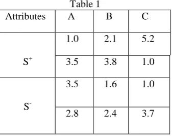
Table 1

Attributes A B C 1.0 2.1 5.2 S+ 3.5 3.8 1.0

S

3.5 1.6 1.0 2.8 2.4 3.7

Let us consider TABLE 1, containing a set a S+ of positive observations and a set S- of negative observations having the attributes A, B and C. To be more specific, we can consider a phenomenon S asbreast cancer and the attributes A, B and C may represent lump size, bone density and age of the person respectively.

Let us first introduce the following cut-points ℧A = 3.0, ℧B = 2.0 ℧C = 3.0

for the attributes A, B and C respectively. These cut-points convert numerical attributes into binary values. Consider an observation α = (αA, αB, αC…) which is mapped to a binary vector y(u) = (yA, yB, yC,…) by assigning

yA = 1, iff αA> ℧A , yB = 1, iff αB> ℧B and yC = 1, iff αC> ℧C for all observations [2][3]. The result of this

binarization of Table 1 is given in Table 2.

Table 2

Boolean Variables

A

B

C

T: true points

0

1

0 F: false points

1

0

1

Multiple cut-points can be introduced for each numerical attribute such that if K-cut-points are assigned, then the attribute A is converted to a K-dimensional Boolean vector.

IV. SUPPORT SET MINIMIZATION

(4)

484 | P a g e

Different methodologies have been proposed to select a small support set such that there is no loss of information following the elimination of the redundant attributes. One of the interesting approaches to avoid the loss of information is to evaluate the quality of each attribute [4]. This evaluation determines the selection of binary attributes to form the support set.

Another simple approach to identify a minimal support set is based on correlation analysis which includes identification of the relationship existing between the attributes. This relationship or connection between two or more attributes is known as correlation and is measured through correlation coefficient.

One way to minimize the support set involves computing the correlation coefficient of each attribute with the result variable. The attribute can be eliminated if value of its correlation coefficient is less than the given threshold value. Other way comprises of calculating the correlation coefficient of each attribute with all the other attributes to obtain a minimized support set. All those variables which are correlated above a threshold with each other are removed and replaced by a single variable. The value of the new attribute is given by the weighted average of the values of each attribute, here weight of each attribute is the correlation coefficient of that attribute with the result.

V. PATTERN GENERATION

The key concept of logical analysis of data is pattern. A pattern is defined as a combination of attribute values that occur together only in some observations. A positive pattern P+ covers at least one positive observation but no negative ones, and a negative pattern P- has a similar definition. So, a combination of patterns is selected such all the examples are covered by at least one pattern.

A hybrid bottom-up─top-down approach is used for pattern generation. In this approach, short patterns are generated by proceeding in a bottom-up fashion; however it could leave some observations uncovered. So, to cover these observations a top-down approach is adopted generating additional patterns that are further simplified by removing literals from them.

A classification rule is generated using a rational combination of patterns which classifies the new observations. In this method, the class of the new observations is determined with the means of the weighted sum of both positive and negative patterns. This weighted sum is known as discriminant.[1][2] Suppose P1, P2,…, Pr are the positive patterns and N1, N2,…., Ns are the negative patterns. The discriminant is given by ∆:

∆ = ∑ ωk+ Pk + ∑ωl- Nl (1)

There are multiple ways of assigning non-negative (non-positive) weights to positive (negative) patterns. The simplest approach is to assign equal weights to all patterns thus giving equal importance to them. However,the weight of a pattern can also be determined by the number of observation points covered by it. The consideration of the degree of pattern as a criterion for assigning weight is another reasonable approach to realize the relative importance of patterns.

(5)

485 | P a g e

VI. RESULTS

This section consists of numerical experiments with the use of proposed approach .A number of experiments are performed on publicly available datasets to make comparisons with the standard LAD

algorithm. In this comparisons are over number of attributes, types of attributes and number of operations. Wisconsin Diagnostic Breast cancer data set, Haberman‟s Survival Data Set, Australian Credit Card are some of the datasets used for the performance analysis of the proposed approach. A subset of the available information (training set) is used for the computation of patterns, thus formulating a classifier which is then evaluated against the training set. A brief description of the datasets from UCI repository is given below.

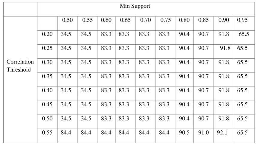
6.1 Wisconsin data set: This data set consists of a total of 569 observations with 32 attributes. Out of 32 attributes, 30 attributes are real valued input features which explain the patient‟s medical profile. There are total of 357 benign case and 212 malignant in the data set.

Table 3 and Table 4 describes the accuracy of the above specified data set, having attributes ID number, diagnosis, radius, texture, perimeter, area, etc smoothness, compactness, concavity, concave points, for different values of correlation coefficient and min-support value. Each row represents accuracy value of LAD tool for fixed correlation and different min-support values when we are using Correlation with Result and Correlation within Attributes respectively, to reduce the support set.

Table 3 Accuracy (Correlation with result) (Data Set 1) Min Support

Correlation Threshold

(6)

486 | P a g e

Table 4 Accuracy (Correlation within Attributes) (Data Set 1)

Min Support

0.50 0.55 0.60 0.65 0.70 0.75 0.80 0.85 0.90 0.95 0.5 62.4 35.2 94.9 94.9 94.9 94.9 94.9 94.9 94.9 34.8 0.6 62.4 35.2 94.9 94.9 94.9 94.9 94.9 94.9 94.9 34.8 0.7 68.5 93.6 94.6 94.6 95.6 95.6 95.6 95.6 95.6 34.8 0.8 89.7 35.3 90.1 90.1 90.1 84.3 87.4 89.6 89.7 34.8 0.9 87.6 80.5 79.2 79.2 79.2 86.7 86.7 39.2 37.2 34.8

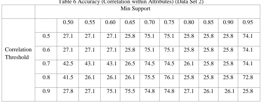
6.2 Haberman’s Data set: The data set contains cases from a study that was conducted between 1958 and 1970 at the University of Chicago‟s Billings Hospital on the survival of patients who had undergone surgery for breast cancer. . This data set records a total of 306 observations. The attributes include age of patient at time of operation (numerical) patient‟s year of operation (year - 1900, numerical), number of positive auxiliary nodes detected (numerical) and survival status (class attribute).

Table 5 and Table 6 describe the accuracy of the above specified data set, having attributes patient‟s age, year of operations, survival status, number of positive auxiliary nodes, etc for different values of correlation coefficient and support value. Each row represents accuracy value of LAD tool for fixed correlation and different min-support values when we are using Correlation with Result and Correlation within Attributes respectively, to reduce the support set.

Table 5 Accuracy (Correlation with Result) (Data Set 2) Min Support

(7)

187 | P a g e

Table 6 Accuracy (Correlation within Attributes) (Data Set 2) Min Support

0.50 0.55 0.60 0.65 0.70 0.75 0.80 0.85 0.90 0.95 0.5 27.1 27.1 27.1 25.8 75.1 75.1 25.8 25.8 25.8 74.1 0.6 27.1 27.1 27.1 25.8 75.1 75.1 25.8 25.8 25.8 74.1 0.7 42.5 43.1 43.1 26.5 74.5 74.5 26.1 25.8 25.8 74.1 0.8 41.5 26.1 26.1 26.1 75.5 76.1 25.8 25.8 25.8 72.8 0.9 27.8 27.1 75.1 75.5 74.8 74.8 27.1 26.1 26.1 25.8

VII. CONCLUSION

The tool is tested on various datasets, some of which are explained above. In general, both the support set minimization techniques produce good results, with the individual best case accuracies averaging in the range of 80-90%. First of all, using correlation with result method, low values of correlation threshold leads to inclusion of unimportant attributes during pattern generation which in turn results in removal of important attributes that might contain some noise or error in them. So again, the accuracy decreases, the best case results occur in the mid-range, which actually differs from dataset to dataset depending on the correctness and relevance of the provided attributes. Secondly, in the case of correlation within attributes increasing the threshold to really high values results in the hampering of any merges, and keeps the original binarized attributes almost intact, thus preventing the loss of useful attributes.

VIII. ACKNOWLEDGEMENTS

The authors are grateful to teachers of Galgotia‟s College of engineering and technology particularly, Mr. Lucknesh Kumar and Mr. Manish Singh for their constant support and guidance to the implementation of work.

REFERENCES

[1] E.Boros, P.L. Hammer, T.Ibaraki, and A.Kogan (1997), Logical analysis of numerical data. Mathematical Programming,79(1-3):163-190.

[2] E.Boros, P.L.Hammer, T.Ibaraki and A.Kogan, An implementation of logical analysis of data,IEEE transactions on knowledge and data engineering Vol.12, No. 2, March/April 2000

[3] G. Alexe, S.Alexe, T.O.Bonates, A.Kogan, Logical Analysis of Data – a vision of P.L.Hammer.Annals of Mathematics Artificial Intelligence, April 2007, Volume 49