Simulation Modelling and Parametric Synthesis of Metal Working Machine Tools Mechatronic Systems of Surface Generation

(1)

Simulation Modelling and Parametric Synthesis of Metal Working

Machine Tools Mechatronic Systems of Surface Generation

Vladimir Molodtsov1,*, János Takács2, Zoltán Párkányi3, and Alexey Isaev1

1

Moscow State Technological University "STANKIN", RU-127055, Moscow, Russia 2

Budapest University of Technology and Economics, HU-1111 Budapest, Hungary 3

Csepel Holding PLC, HU-1211 Budapest, Hungary

Abstract. This paper presents the principles of the designing metal working machine tools mechatronic systems of surface generation which are optimal from the point of view of reproducing given part profiles. It is shown that the degree of their optimality is determined by the proximity of their characteristics to the frequency characteristics of an ideal low-pass filter. Mathematical methods for building compact mathematical models of the drive hardware, adequately describing the inertial and elastic characteristics of the elements of its structure, is described. These models are convenient for simulating control loops of the machine tools feed drives. A method for the parametric synthesis of a two-mass mathematical model of a subordinate control system for a feed drive with an elastic-dissipative coupling between equivalent lumped masses which simulate a moving unit and rotating elements of the drive mechanism is proposed. The synthesis problem is reduced to solving a system of nonlinear equations. Examples to demonstrate the proposed methods and models capabilities are given.

1 Feed drives design optimization

criterion

Increasing productivity and ensuring high precision machining of parts are priority areas for improving metalworking machines. Part profile is the result of coordinated motions of tool and workpiece. In the CNC machine tools mechatronic systems of surface generation, the feed drives are the crucial elements which ensure coordination of their motions. They receive their job via information network of the controller. The change from mechanical links to data communication allowed to increase the equipment flexibility and part profile variety significantly, while simultaneously increasing the machining accuracy, due to the exclusion of the influence of the error of the mechanical links of kinematic chains which provide mortions coordinations in the manually operated machine tools [1–4]. However, axis drives errors and the information network latency have direct impact on the part accuracy.

The relationship between movements of the machine components along generalized coordinates and paths of tool and workpiece relative motion is determined by dependencies:

r t_д

( )

= f

(

{

r

_вых

( )

t

}

)

(1)

and

{

( )

}

1

(

( )

)

вх t f r to

r ₌ −  _, ₍₂₎

which are formalism for direct and inverse kinematics. Here r x y z_д

(

_i, _i, _i

)

and r x y zo

(

j, j, j

)



are radius-vectors

of corresponding points of a part and an image in the global coordinate system Oxyz,

( )

{

}

1

( )

,...,

( )

T

вх вх

вх t q t qm t

r _{= } _ and

{

r_вых

( )

t

}

=

( )

1 ,...,

T вых вых

m

q t q t

 

=   are input and output vectors of

the machine generalized coordinates associated with

drives 1,…,m, t is a scalable parameter (time). The

relation between input and output vectors of the machine generalized coordinates is:

{

r_вых

( )

t

}

= f

(

{

r_вх

( )

t

}

)

. (3)

The analysis of expressions (1) to (3) allows us to identify the main directions of improving the accuracy of contouring. We can vary system of surface generation, transfer functions of drives and the control signal. However, all of these are by some means or other depend on the characteristics of the machine tool drives.

(2)

However, the time delays between output and input signals in the machine drive do not play such a significant role as in the classic servo. It is enough to ensure the unit values of the transfer function modules, the equality of the time delays of the drives which are the components of the machine system of surface generation, and the equality of the time delays of the components of the output signal spectrum in the range of frequencies of the control signal in order to reproduce it without distortion.

The condition of undistorted drive response to an arbitrary input signal along the i-th generalized coordinate is:

q

_iвых

( )

t

=

q

_iвх

(

t

−

t

_i

)

, (4)

where ti ≥ 0 is time delay (group-delay distortion) at a

given coordinate. Drive specifications must match those of an ideal low-pass filter. If 0≤ ≤ω 2πf₀ then its

frequency response and phase response are A

( )

ω =1

and Φ

( )

ω

= −

tω

accordingly, where

( )

d d const

t

= − Φ

ω

= , and f0 is cut-off frequency.

Since it is impossible to implement an ideal filter, the transfer function of each drive is to be searched for among the filters whose frequency characteristics are the best approximations of the useful component of the input signal that is ideal in the frequency range [5,6].

A straightforward decision is to choose a single reference transfer function W s_э

( )

, that satisfies the expression

{

r

_вых

( )

t

}

≈L−1

(

W s_э

( )

{

r

_вх

( )

s

}

)

, (5)

a function that will ensure compliance with the requirements specified above and the subsequent structural and parametric synthesis of the corresponding drives.

2 Modeling drive mechanisms

The elastic properties and inertial characteristics of the mechanism have a significant effect on the dynamic processes in the feed drive, since the resonance phenomena arising in the mechanism impede the effective adjustment of its contours. Despite its importance, this problem is under-examined.

Fig. 1. Test bench.

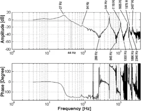
The analysis of the results of experiments conducted

at the test bench (Fig. 1), showed that the frequency

response spectrum of its speed loop taken from the motor sensor has a complex composition with a large number of resonance peaks, most of which are outside the loop bandwidth in the frequency range of 50 to 2500 Hz (Fig. 2).

Here you can also see the dips corresponding to the speed loop transfer function zeros. An increase in the gain of the controller is accompanied by the speed loop bandwidth widening and increasing of the amplitudes of the oscillations at frequencies outside of the bandwidth (Fig. 3). A further gain increase leads to a loss of circuit stability.

Fig. 2. Poles and zeros of the frequency response of the speed loop.

Fig. 3. The influence of the gain of the speed loop on its frequency response.

(3)

Simulation of the rotating components of the drive was performed with the ANSYS finite element analysis

software (see the model layout in Fig.4). Waveforms of

the torsional oscillations of mechanical components of the drive with a free and fixed rotor are shown in Fig. 5.

a)

b)

c)

Fig. 5. Waveforms of torsional vibrations at natural frequencies: a) – 593, b) – 1262 and c) – 1885 Hz. Lines are the simulation results obtained in ANSYS (solid line: the original model, natural frequencies without brackets; dotted line: model with a fixed motor rotor, natural frequencies in brackets). Markers are chain models.

The finite element model of the rotating component of the feed drive mechanism cannot be used directly to model its control loops, because of its bulkiness, redundancy and closeness.

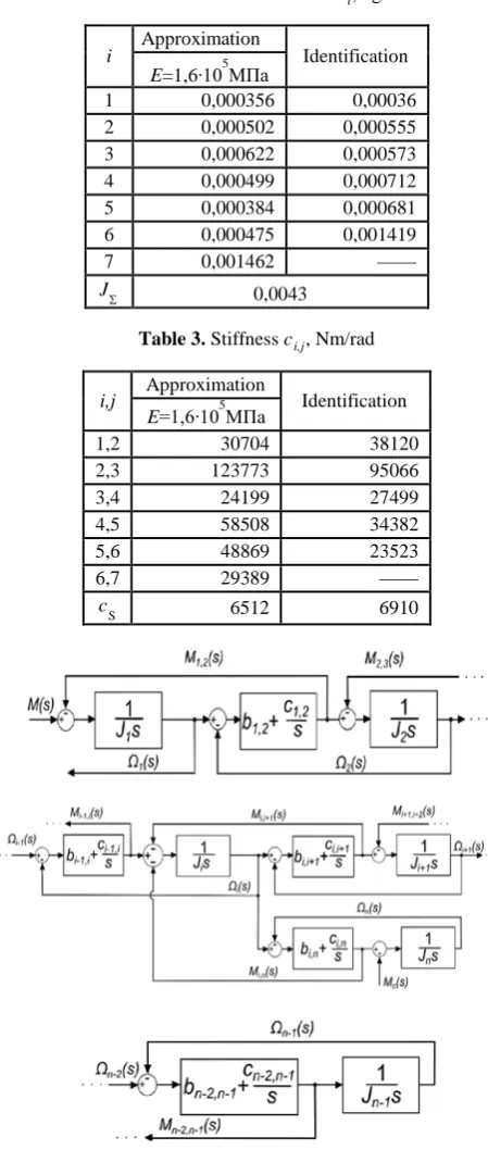
Fig. 6. Block diagram of the discrete model of the mechanical parts of the drive.

The most convenient for these purposes are discrete

models shown in Fig. 6, which provide a satisfactory

description of dynamic processes in the mechanical part

with minimal resources [7,8]. Using this approach, we build a system

( )

2

1 1 1,2

2

2 2 1,2 2,3

2

1 1 2, 1 1,

2

1, , 1 ,

2

1 1 , 1 1, 2

2

2 2 3, 2 2, 1

2

1 1 2, 1

2

,

i i i i i i

i i i i i i+ i n

i i i i i i

n n n n n n

n n n n

n n i n c

J s s М s М s

J s s М s М s

J s s М s М s

J s s М s М s М s

J s s М s М s

J s s М s

J s s М s М s

ϕ ϕ

ϕ

ϕ ϕ ϕ

− − − − −

−

+ + + + +

− − − − − −

− − − −



= −



= − _

 

= − _

= − −



= −

=

= −



       

(6)

of n equations in operator form. Here J

1 … Jn–1 are

equivalent moments of inertia of the rotating components of the mechanism, J

n is equivalent moment

of inertia of the translational component (table),

( )

i s i s s

ϕ

= Ω are angles of twist of the drive

elements at the points of location of the corresponding

reduced masses. Equivalent moments caused by elastic

deformations and internal friction in the drive elements between the reduced masses are given by expressions of the form: M_{i k}_,

( )

s =

(

b s_{i k}_, +c_{i k}_,

)

_ϕ_i

( )

s −ϕ_k

( )

s _, where c

i,k and bi,k are torsional stiffness and damping factor of

the respective part of the mechanism, M(s) and M

c(s) are

torques of the motor and the resistance forces.

а)

b)

Fig. 7. Block diagrams of discrete chain systems: a) with free motor rotor; b) with fixed motor rotor.

When analyzing the expressions for angles of twist of the first

( )

1 , 1

1 1

1

n l l

n l

c

n n

k s

G s

s M s М s

G s G s

ϕ

− +

− =

= −

∏

, (7)

where

( )

2

( )

1 1 1,2 1 1,2 2

n n n n

G s =J s G − s +k s G− s −k s G− s ,

and the second

-1,00 -0,80 -0,60 -0,40 -0,20 0,00 0,20 0,40 0,60 0,80 1,00

0 250 500 750 1000 1250 мм

-1,00 -0,80 -0,60 -0,40 -0,20 0,00 0,20 0,40 0,60 0,80

0 250 500 750 1000 1250 мм

-0,60 -0,40 -0,20 0,00 0,20 0,40 0,60 0,80 1,00

(4)

( )

_{( )}

( )

_{( )}

( )

1 , 1

1,2 2 2

2 1

1 1

n l l

n l

c

n n

k s

k s G s

s s М s

G s G s

ϕ ϕ

− +

− =

− −

= −

∏

, (8)

where

( )

2

( )

1 1 1,2 2 2,3 2

n n n

G₋ s =_J s +k s _G₋ s +k s G₋ s −

( )

2,3 n 3

k s G− s

− _, mass chain model shown in Fig.7a , it

was found that the zeros of its transfer function correspond to the poles of the fixed rotor system (Fig. 7b). Here, G_n(s), G_n-₁(s), G_n-₂(s) and G_n-₃(s) are characteristic polynomials of chain systems of dimensions n, n–1, n–2 and n–3.

To find a relation between the finite element models of torsion systems and the chain models shown in Fig. 7, let’s consider the peculiarities of formulating the eigenvalue problem for them. Neglecting damping, let’s represent the model of the chain system (Fig. 7a), in matrix form:

(

[ ]

_i

[ ]

)

{ } { }

0

i

x E

α − Ψ = , (9)

where

[ ] [ ] [ ][ ]

1 2 1 2

n M C M

α − −

=

 , [M] и [C] are matrices

of masses and rigidity,

{ }

[ ] { }

1 2

i M i

Ψ = Φ , x_i and

{ }

[

1

]

T n

i

Φ = Φ  Φ are i-th eigenvalue and vector. Elements of the tridiagonal matrix

[ ]

1

1 1 2

3 2 2 1

2 1 1

0 0

m m m

m m m m

n

α α α α α α α α

α α α α α α α

−

− − −

 − 

 

− +

 

=  

 ₊ ₋ 

 

 − 

 

 

     

 

(10)

are squares of partial frequencies where

α

_j =c_{l l}_,₊₁ J_i , where j=1,…,m (m=2n–2). The partial frequency squared

matrix of a system with a fixed rotor

[ ]

1 n

α ₋ is obtained

from it by deleting the last row and column.

In solving the eigenvalue problem, an important advantage of symmetric tridiagonal matrices is the relative simplicity of finding the coefficients of the characteristic polynomial, which is used in some algorithms in the final stage of finding eigenvalues [9,10]. A characteristic polynomial of a system (9) with a symmetric general tridiagonal matrix is recursively determined by the sequence of polynomials

fr

( )

x =(ar−x f) r−₁

( )

x −b fr2 r−₂

( )

x , (11)

where ar and br where ar and br are the corresponding

diagonal and off-diagonal elements of this matrix,

2,...,

r= n. Assuming f₀

( )

x =1 and f1

( )

x = −a1 x_{, we}

obtain the sequence of polynomials known as the Sturm sequence [9]. Each of these polynomials is a characteristic polynomial of the matrix

[ ]

1 2

2 2

1

0 0

r

r r

a b

b a

a b

b a

α

−

 

 

=

 

 

 

    

 

,

where r=1,...,n, which can be written as

( ) ( )

( )

1 ( )

( )

2 ( ) 2

0 1 2

1r r 1r r 1r r

r

f x = − d + − − d x+ − − d x +

−d_r( )−r₁xr−1+xr. (12)

The coefficients of the characteristic polynomialf_r

( )

x

are expressed in terms of the coefficientsar and br of the

matrix

[ ]

α

_r and the coefficients of the characteristic

polynomialsf_r₋₁

( )

x and f_r₋₂

( )

x of matrices

[ ]

1 r

α ₋ and

[ ]

α

r−2 by means of recurrent dependences [10].

Taking into account the structure peculiarities of the

matrix

[ ]

α n_{, the scheme of finding the coefficients of its}

characteristic polynomial the scheme of finding the coefficients of its characteristic polynomial f_n

( )

x takes the form:

d_n( )n−₁=d_n(−n₂−1)+

α

₁;

d_n( )n−₂ =d_n(n−₃−1)+

α

₁d_n(n−−₂1)−

α α

₁ ₂;

d_n( )−n₃=d_n(−n−₄1)+

α

₁d_n(n−−₃1)−

α α

₁ ₂d_n(n−−₃2);

………. (13) d₂( )n =d₁(n−1)+

α

₁d₂(n−1)−

α α

₁ ₂d₂(n−2);

d₁( )n =d₀(n−1)+

α

_{1 1}d(n−1)−

α α

₁ ₂d₁(n−2);

d₀( )n =

α

₁d₀(n−1)−

α α

₁ ₂d₀(n−2)=0.

Here d_l(n−1) are the coefficients of the characteristic

polynomial of a positive definite matrix

[ ]

1 n

α ₋, obtained

from

[ ]

n

α by the deletion of the n-th row and n-th

column, and d_l(n−2)are the coefficients of the

characteristic polynomial of a positive definite matrix

[ ]

α

n−2, obtained from

[ ]

α n−1 by the deletion of the

(n–1)-th row и (n–1)-th column.

Assuming d_l( )n and d_l(n−1) are known, we convert the scheme (13) into the form

( ) ( 1)

1 1 2

n n

d d

α

−

− −

=  − _;

( 1)

(

( ) ( 1)

)

( 1)

2 2 3 1 2 2

n n n n

d ₋− = d₋ −d₋− α =d ₋− −α ;

( 1)

(

( ) ( 1)

)

( 1) ( 2)

3 3 4 1 3 2 3

n n n n n

d −− = d − −d −− α =d −− −α d −− ;

………..

( 1)

(

( ) ( 1)

)

( 1) ( 2)

2 2 1 1 2 2 2

n n n n n

d − = d −d − α =d − −α d − ;

( 1)

(

( ) ( 1)

)

( 1) ( 2)

1 1 0 1 1 2 1

n n n n n

d − = d −d − α =d − −α d − ;

( ) ( 1) ( 2)

0 0 2 0 0

n n n

(5)

Here d_l(n−1) are the coefficients of the characteristic

polynomial of a positive semi-definite matrix

[ ]

1 n α ₋ ,

obtained from

[ ]

1 n

α ₋ by equating α₂ to zero.

From the first two dependencies of the newly formed scheme, we can determine the squares of the partial

frequencies α₁ and α₂. From the last (n–1) of its

dependencies we obtain the coefficents d_l(n−1), and from

the last (n–2) of its dependencies we obtain d_l(n−2). Thus, the coefficients of the characteristic polynomials of the matrices

[ ]

α _n₋₁ and

[ ]

α

_n₋₂ are recurrently expressed in terms of the coefficients of the characteristic polynomials of the matrices

[ ]

α

 _n and

[ ]

α _n₋₁. Applying this scheme, we can consistently calculate all squares of the partial frequencies of the matrix (10) from α₁ to α_m_–

2.

It is more convenient to divide the computational procedure into (n–2) cycles; within each of them we will perform the same steps. The computational algorithm in the i-th cycle, where i=1,…,n–2, can be represented as:

Step 1. ( 1) ( )

2 1 1

n i n i i dn i dn i

α

− + −

− = − − − −

Step 2.1) ( )

(

( 1) (1 )

)

2 1

n i n i n i

l l l i

d − = d − + −d₋− α ₋

Step 3.

α

₂_i=d_{n i}(n i_{− −}−)₁−d_{n i}(n i_{− −}−₁) (14)

Step 4. 2) 3) ( 1)

(

( ) (1 )

)

2

n i n i n i

l l l i

d − − = d − −d₋− α

Step 5. d₀(n i− −1)=d₀( )n i−

α

₂_i

1) This operation is performed l=1,…,n–i–1 times in each cycle.

2) This operation is performed l=1,…,n–i–2 times in

each cycle.

3) If i =n–2, step 4 is skipped.

For the matrix

[ ]

2

α

 the scheme of finding the

coefficients of its characteristic polynomial takes f₂

( )

x

the form [10]: d₁( )2 =d₀( )1 +

α

_m₋₁ and

( )2 ( )1

0 m 1 0 m 1 m 0

d =

α

₋d −

α α

₋ = . Assuming d₁( )2 and d₀( )1 are known, we obtain the dependencies for the last two squares of partial frequencies

α

_m =d₀( )1 (15,а)

and

α

_m−₁=d₁( )2 −d₀( )1 . (15,b)

The roots pi and ziare related to the coefficients of

the characteristic polynomials of the matrices

[ ]

α

 _n and

[ ]

α n−1 by dependencies called Vieta’s formulas. Since

the calculation of the coefficients of high-order polynomials with them is fraught with significant computational difficulties, we use Newton's formula for this purpose to determine the power sums of the roots of a polynomial

( ) ( )

1 ( ) 1

_{( )}

1

_{( )}

( )

1

1 1

k

k r l r

k i r k k l i r l

l

s x kd s x d

−

− −

− − −

=

= − +

∑

− , where

( )

1 r

k

k i i

i

s x x

=

∑

, where is the power sum of the degreek

of r roots of the polynomial (12), d_k( )r are the

coefficients of the polynomial (12), 1≤ k ≤ r. The

coefficients of the characteristic polynomial in the Leverrier method are found in the same manner. Recurrent relations for the calculation of the coefficients of characteristic polynomials of matrices

[ ]

α

 _n и

[ ]

α _n₋₁ have the form

( )

1 1

1 1 1

1 k

l n

k i k l i n l

n l

n k k

s p s p d

d

k − ₋

− −

=

− −

=

−

∑



 _(16,a)

and

( )

1

1 1

1

1 1

1

1 k

l n

k i k l i n l

n l

n k k

s z s z d

d

k

− ₋

− − − −

− =

− − −

− −

=

−

∑

, (16,b)

where k=1,…,n–1;

( )

1 r

k

k i i

i

s p p

=

∑

;

( )

1 r

k

k i i

i

s z z

=

∑

.

Consequently, in order to calculate the coefficients

α₁,…,α_m, which are the squares of the partial

frequencies of the chain systems, the block diagrams of

which are shown in Fig. 7, we have to solve two

problems about the eigenvalues of dynamic systems obtained as a result of finite element modeling of the mechanical component of the drive (the second system

has a motor with a fixed rotor). Then, using n–1 lower

eigenvalues (without taking into account zero), calculate the coefficients of the characteristic polynomials of the

matrices

[ ]

n

α

 and

[ ]

1 n

α ₋ . After that, using the scheme

(14) and the dependences (15), calculate α₁,…,α_m. The relationship between the (2n–2) squares of partial frequencies and unknown (n moments of inertia and (n–1)-th stiffness) is given by dependencies of the form

α_j=c_{l l}_,₊₁ J_i . (17)

The relationship between the indices in (17) is given by the expressions

i= j 2 1+ (18,а)

and

l=

(

j+1 2

)

, (18,b)

where 1≤ ≤i n, 1≤ ≤ −l n 1 и 1≤ ≤j 2n−2. In these expressions, the division operation is to considered as an integer.

(6)

free parameter (the value of which is to be determined using additional information). For convenience of calculations, we can choose J1.

Table 1. Relationship between the indices of the squares of partial frequencies, moments of inertia and stiffness.

j i (see (18,а)) l (see (18,b))

1 1 1

2 2 1

3 2 2

4 3 3

… … …

2i–3 i–1 i–1

2i–2 i i–1

2i–1 i i

2i i+1 i

… … …

2n–5 n–2 n–2

2n–4 n–1 n–2

2n–3 n–1 n–1

2n–2 n n–1

Using expressions (18), we build the correspondence

table of indices 1. It follows from it that in equations

(17), two different partial frequencies correspond to one moment of inertia or rigidity of the model. This correspondence is violated only for the first and last mass. Using it, we get from the relationship between α₂_i_–

3 and α2i–2 we obtain

2 3 1 2 2

i

i i

i

J α J

α − −

−

= . Using this

dependence, we can recurrently express the moments of inertia of all rotating masses in terms of the moment of inertia of the first one. The expression relating the i-th moment of inertia to the first one, is:

2 3 1

2 2 2 k i

k i

k k

J J α

α

= − = −

=

∏

. (19,a)

Similarly, from the relationship between α₂_i_–1 and α₂_i_–2

we obtain 2 1

, 1 1,

2 2 i

i i i i

i

c α c

α −

+ −

−

= and

2 1

, 1 1 1

2 2 2 k i

k i i

k k

c Jα α

α

= − +

= −

=

∏

, (19,b)

and the relationship between the moment of inertia of the first disk and the stiffness of the elastic element associated with it is given by the expression

c_1,2=α₁J₁. (19,c)

Let’s express the total moment of inertia of the chain system in terms of the moment of inertia of the first body

2 3 1

1 2 2 2 2

1

n n k i

k i

i i k k

J J α J

α

= − Σ

= = = −

  

= = +_ _ __

 

 

∑

∑ ∏

.

Since we can easily obtain information about the total moment of inertia of the rotating components of the drive using a solid modeling system, we will use this dependence to find the free parameter. The expression for calculating the moment of inertia of the first body is:

2 3 1

2 2 2 2

1

n k i k

i k k

J J α_α

= − Σ

= = −

  

= _ + _ __

 



∑ ∏

. (20,a)

The total rigidity of the chain system can also be expressed in terms of the moment of inertia of the first body

1

2 2 1 1

2 2 2 1 1

n k i k i k k

c α J α

α

− = − Σ

= = −

 

= _ + _



∑∏

. (20,b)

Step one. Considering the obtained results, the

method for determining unknown values of the moments of inertia of lumped masses and stiffnesses of elastic bonds of system (9) can be divided into 4 steps.

Nonzero eigenvalues of the rotating components of the drive with a free (poles pi) and a fixed rotor (zeros zi).

Step two. Using nonzero eigenvalues of the poles

and zeros, using the recurrence dependences (16) obtained from Newton's formulas for determining power sums of the roots of the polynomial, the coefficients of the characteristic polynomials (12) of the tridiagonal square matrixes of partial frequencies of systems with a free and fixed rotor are determined.

Step three. From the characteristic polynomials of

these tridiagonal matrices coefficients obtained at Step two, the squares of partial frequencies are found using the computational procedure consisting of (n–2) cycles, within the framework of each of which the same steps described by the recurrence dependences (14) are performed.

Step four. Unknown moments of inertia of

concentrated masses and stiffness of elastic bonds are determined by formulas (20) based on information about the total moment of inertia of the rotating elements of the drive hardware.

(7)

Table 2. Moments of inertia J_i, kg∙m2

i Approximation Identification

E=1,6∙105МПа

1 0,000356 0,00036

2 0,000502 0,000555

3 0,000622 0,000573

4 0,000499 0,000712

5 0,000384 0,000681

6 0,000475 0,001419

7 0,001462 ––––

J_Σ _0,0043

Table 3. Stiffness c_i,j, Nm/rad

i,j Approximation Identification

E=1,6∙105МПа

1,2 30704 38120

2,3 123773 95066

3,4 24199 27499

4,5 58508 34382

5,6 48869 23523

6,7 29389 ––––

c

S 6512 6910

Figure 8. Multi-mass simulation model of the feed drive hardware.

Fig. 9. Comparison of experimental data with simulation results ( simulation results, experimantal data).

To obtain the frequency characteristics of the drive, a

model of its hardware shown in Fig. 8 was used, which

in combination with a rather simple model of drive control loops forms a mathematical model of a dynamic system of a multiloop feed drive.

Fig. 9 shows a comparison of the simulation results

obtained in the MATLAB environment with experimental frequency characteristics of the drive.

3 Parametric synthesis

Unlike torsional vibrations, the natural frequencies of the axial vibrations of the translational component are either within the bandwidth of the position loop or in close proximity to it and have a direct effect on the quality of machining. If the torsional stiffness of the rotating elements of the drive can be neglected, the entire drive hardware can be represented as two rotating masses that

simulate a translational component and drive

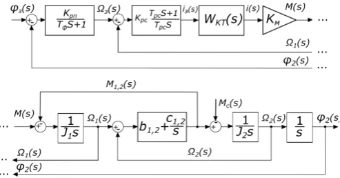
mechanisms brought to the motor shaft, and an elastic-dissipative coupling between them. For this case, the block diagram of the closed-loop feed drive with current,

speed and position loops, is shown in Fig. 10. On this

diagram, W_кт

( )

s ≈1

(

T T s_m _min 2+T s_min +1

)

is the transfer function of the optimized current loop [11], Tm and Tmin

are the basic and short time constants, kM is the

electromechanical constant of the motor, J1 and J2 are

the reduced moments of inertia of all rotating elements of the mechanism and the translational unit, c_1,2 is the axial stiffness of the traction device,b_1,2– is the friction in the structural elements of the drive.

(8)

Fig. 10. Block diagram of a feed drive with a two-mass hardware closed by position, speed and current.

In the drive loops, a typical PI speed controller with a gain ratio kрс and a time constant Tрс, a proportional position controller with a gain ratio k_рп and a filter in the speed reference circuit where T_ф=T_рс is the filter time constant, are used. The main variables of the model are

plotted on the diagram: ϕ_з(s) and ϕ₂(s) are the

reference angle and the reduced angle of rotation of the translational unit, respectively; Ω_з(s) and Ω₁(s) are the

preset and actual motor speeds; Ω₂(s) is the reduced

speed of the moving unit; i_з(s) and i(s) are the preset and actual current in the motor windings; M(s) and Mc(s) are

the moment of motor and the moment of resistance;

M1,2(s) is the moment caused by elastic deformations

and internal friction in the drive elements between the reduced masses.

The dependence of the reduced angle of rotation of the moving unit on the reference angle and the moment of resistance corresponding to this scheme has the form:

ϕ

₂

( )

s =Wϕ ϕ₂ _з

( ) ( )

s

ϕ

_з s −Wϕ₂_Mс

( ) ( )

s M_c s , (21)

where

( )

1,2 1,2 2

1,2 1,2 з

b s c

W s

c G s

ϕ ϕ ϕ + = ,

( )

2 1,2 1,2 Мс Mc H s W s

с G s

ϕ

ϕ =

and

( )

1,2

(

2

)

1 2 1,2

1,2 1,2

1 1

рс

Mc min min

рп M рc

T c J b

s

H s T T s T s s s

k k k m c c

   =  + + _ + + +_     1 рс

T s 

+ _{+ }.

The characteristic polynomial of the transfer functions of system (21) is of the form:

( )

1 2 7

1,2

1,2 min рс

M рc рп

T T T J J

G s s

k k k c

m

ϕ = +

1 2 1 2 6

1,2

1,2 1 2

1 min рс

M рc рп

T T J J J J

T b s

k k k c m J J

 + 

+ _ + _ +

 

1 2 1 2 1 2 5

1,2 1,2

1,2 1 2 1 2

1 рс

min min

M рc рп

T J J J J J J

T T c T b s

k k k c m J J J J

 + + 

+ _ + + _ +

 

(

1 2

) (

1 2

)

1,2 2 4

1,2 1,2 рс min

рп M рc M рc

T T J J J J b J

s

k k k k k c c

 + + 

+  + +  +

 

 

(

1 2

)

1,2 2 3

1,2 1,2

1 рс

рс рп M рc

T J J b J

T s

k k k c c

 + 

+  + +  +

 

 

1,2 2 1,2

1,2 1,2 1 1 1 рс рп рп b b

T s s

k c k c

 

+ _ + _ +_ + _ +

   

(22)

If we design the drive mechanism, power unit and control system simultaneously, it is possible to vary the entire design considering the limitations caused by energy feasibility, which provides an intangible advantage in finding solution to the problem.

The parametric drive synthesis is based on equating the coefficients of the characteristic polynomial (22) of system (21) to the coefficients of the reference polynomial

( )

7 6 5 4 3 2

7 6 5 4 3 2 1

ˆ ˆ ˆ ˆ ˆ ˆ ˆ 1

Э

G sν =a sν+a sν+a sν+a sν+a sν+a sν+a sν+

,

(23)

selected from the considerations outlined above. Before equating, the coefficients of polynomial (22) are reduced to a dimensionless form by changing variables

s

=

ω

_{ν ν}

s

,

where n_a₀

ν

ω = is the technical constant having the

frequency dimension.

Let us introduce the new variables

T

_J

=

J

₁

(

k k

_M _рс

)

,

2 1,2 с

T = J c ,

T

b

=

b

1,2

c

1,2,

T

рп

=

1 k

рп and

(

1 2

)

1

J

k = J +J J . After changing the variables in (22)

and equating the coefficients for the corresponding degrees of the polynomials, we obtain the following system of equations:

(

)

(

)

(

)

(

)

(

)

(

)

2 7 7 2 6 6 2 5 5 2 4 4 2 3 3 2 2 1 ˆ ˆ ˆ ˆ ˆ ˆ ˆ min J рc c рп

min J рc рп J b c

J рc рп J min J min b c

рc рп J min J J J b c

рп J рс J рс b c

рп рс b

рп b

T T T T T T a

T T T T k T T T a

T T T k T T k T T T a

T T k T T k T T T a

T k T T T T T a

T T T a

T T a

m ν m ν m ν ν ν ν ν

ω

 =  + =   + + =   + + = _  + + = _  + = _  + = _

. (24)

Converting the variables Tm, Tmin, TJ, Tрс, Tc, Tb and

T_рп of system (24) into a dimensionless form by

multiplying them by ων, we obtain the following system:

(

)

(

)

(

)

(

)

(

)

2 7 2 6 2 5 2 4 2 3 2 1 ˆ ˆ ˆ ˆ ˆ ˆ ˆ

min J рc c рп

min J рc рп J b c

J рc рп J min J min b c

рc рп J min J J J b c

рп J рс J рс b c

рп рс b

рп b

a

k a

k k a

k a a a m m m

t t t t t t

t t t t t t t

t t t t t t t t

t t t t t t t

t t t t t t

t t t

t t  =  + =   + + =   + + =   + + =   + =   + = _

, (25)

where

t

_m

=

ω

_{ν m}

T

,

t

_min

=

ω

_ν

T

_min,

t

_J

=

ω

_ν

T

_J,

t

_рс

=

ω

_ν

T

_рс,

c ν

T

c

(9)

Equations (25) have 8 variables (t_m, t_min, t_J, t_рс, t_с,

t_b, t_рп and k_J) and an infinite number of solutions. Among the variables, a special place is occupied by the

time constant t_b, since it is related to the damping

coefficient of the traction device, with a poorly predicted value. We consider t_b to be a variable, the admissible values of which can be determined based on additional conditions and the physical meaning of the problem.

Solving (25), we can find the dependencies for calculating the remaining 7 variables. The solution comes down to dependencies

t

_рп =aˆ₁−

t

_b=

b t

₁

( )

_b (26,a)

and

( )

2 2

2 1

1 1

ˆ ˆ

ˆ

b b b

рс

b b

a a a

b t

t t

t

b t

− +

= =

− , (26,b)

and cubic equation

( )

3

( )

2

( )

0

b b b b

A

t

pν+B

t

pν+C

t

pν+E

t

=

,

(26,c)

where

( )

2

(

( )

)

7 2 1

ˆ

b b b b b

A t =at b t −t b t ,

( )

b

B

t

=

(

2 a

ˆ

₇

+

a

ˆ

₆

t t b t

_b

)

_b ₁

( ) (

_b

−

a

ˆ

₇

+

a

ˆ

₆

t b t

_b

) ( )

₂ _b ,

( )

b

С

t

=

a

ˆ

₅

b t

₂

( ) (

_b

−

a

ˆ

₅

t

_b

+

a

ˆ

₆

) ( )

b t

₁ _b and

( )

2

( )

2

b b b

E

t

=

t b t

− −aˆ₃

b t

₂

( )

_b +aˆ₄

b t

₁

( )

_b .

The relationship between the initial set of variables in (26, c) and the auxiliary variable pv is given by

(

)

2

1 2 1,2 1,2 1,2

2 2 2

1 2 1,2

J c

J J c c

k p

J J J

ν

ν ν ν

ω

t ω ω ω

+

= = = = . (26,d)

The remaining dependencies are of the form

(

( )

)

(

)

( )

4 3 2 6 7

2

2 1

ˆ _b ˆ _b _b ˆ ˆ _b

c

b b b

a t a t b t a at p_ν p_ν

t

b t t b t

− − − −

=

− , (26,e)

7

2

6 7

ˆ

ˆ ˆ _J _b _c

a

a a k

m

t

t t

=

− , (26,f)

( )

2

3 2 1

2

ˆ _b _b _b _c

J

b J

a

k

t b t b t t

t

b t

− −

= , (26,g)

min ˆ7 ₂ J рc c п

a

m

t

t t t t t

= . (26,h)

Given the value of the base constant Tm, which

determines the speed of the drive control system, we can go to the initial set of variables of system (24), and then calculate the design parameters of the drive.

An advanced methodology for designing a feed drive with a rolling screw-nut transmission includes 4 stages as follows.

At the first stage, based on information about the

mass, speed of movement of the actuating unit and the

external loads acting on it, the reduction coefficient of the traction device and the complete drive are selected using traditional methods. The components of the drive have the required speed and power characteristics.

At the second stage, based on a requirements

analysis of accuracy and dynamic quality of the equipment, a reference polynomial is selected and a verification of its correspondence with the drive speed is performed. Preliminary estimates of stiffness, moment of inertia of the rotating components and damping of the drive mechanism are calculated.

At the third stage, using the information on the

maximum travel, speed, acceleration and dimensions of the actuating component, the design of the following units is selected: rolling screw-nut transmission, bearings, clutch or additional gearbox. Then, the traction device is designed with evaluation of its rigidity and the moment of inertia of the drive mechanism rotating components. The results are compared with the calculated values. If the difference is significant, changes in the mechanical design are made. For this purpose, a specialized software package is used, which allows performing the calculation of dynamic characteristics and selecting the main structural elements of the designed feed drive in interactive mode.

At the final stage, the Simulink environment

simulates the designed drive. The correspondence between its frequency characteristics and the characteristics of the reference polynomial is checked. Performance and overshoot are estimated. The influence of torsional vibrations in the mechanism on the dynamic characteristics of the drive is analyzed.

The design workflow is iterative. If problems arise, a transition to earlier stages of design is possible.

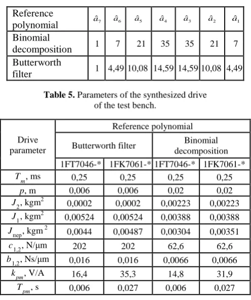
Table 4. Examples of reference polynomials.

Reference

polynomial aˆ7 aˆ6 aˆ5 aˆ4 aˆ3 aˆ2 aˆ1

Binomial

decomposition 1 7 21 35 35 21 7

Butterworth

filter 1 4,49 10,08 14,59 14,59 10,08 4,49

Table 5. Parameters of the synthesized drive of the test bench.

Drive parameter

Reference polynomial

Butterworth filter Binomial decomposition 1FT7046-* 1FK7061-* 1FT7046-* 1FK7061-*

T

m, ms 0,25 0,25 0,25 0,25

p, m 0,006 0,006 0,02 0,02

J₂, kgm2 0,0002 0,0002 0,00223 0,00223

J 1, kgm

2

0,00524 0,00524 0,00388 0,00388

J_пер, kgm 2 0,0044 0,00487 0,00304 0,00351

c

1,2, N/μm 202 202 62,6 62,6

b_1,2, Ns/μm 0,016 0,016 0,0066 0,0066

k_рт, V/A 16,4 35,3 14,8 31,9

(10)

k_рс, As/rad 2,78 4,87 1,62 2,84

T_рc, s 0,0024 0,0024 0,0051 0,0051

k_рп, 1/s 205 205 83,3 83,3

T_ф, s 0,0024 0,0024 0,0051 0,0051

p is screw pitch, J_пер_{– moment of inertia of the rotating parts of}

the traction device.

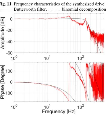
The results of the parametric synthesis of the test bench drive corresponding to the second stage of the design process for two types of motors (1FT7046-* and

1FK7061-*) and reference polynomials from Table 4 are

presented in Table 5. The type and bandwidth of the

frequency characteristics of the position loop shown in

Fig. 11 depend only on the choice of the reference

polynomial and the base constant Tm. Consequently,

choosing the same reference polynomials and complete drives with the necessary speed for all axes, we get the same transfer functions for their position contours. However, it should be borne in mind that the distribution of the moments of inertia of the rotating drive elements forms an unpredictable resonant picture of torsional vibrations. To control this situation, it is necessary to use a full-fledged multi-mass drive model.

Fig. 11. Frequency characteristics of the synthesized drive ( Butterworth filter, binomial decomposition).

Fig. 12. Comparison of synthesis results with experimental data ( Butterworth filter, experimental data).

A comparison of the experimental frequency characteristics obtained after suppressing resonance phenomena in the test bench drive mechanism with the

simulation results (see Fig. 12) allows us to conclude

that, thanks to a rational choice of the design parameters, it was possible to expand the drive bandwidth from 52 to 142 Hz.

4 Conclusions

1. The feed drive mechanism with rolling screw-nut transmission is a complex dynamic object. The resonance phenomena in this unit have a significant impact on the operational characteristics of the entire machine tool. In most cases, the resonance is caused by axial and torsional vibrations of the structural elements of feed drive. The natural frequencies of axial vibrations of the translational unit located in the bandwidth of the position loop from (30–40 Hz to 200 Hz) or in close proximity of it have a direct imact on the quality of machining process. Resonance phenomena during torsional vibrations of rotating structural elements of the traction device (screw, clutch, engine rotor, etc.) occur at frequencies from several hundred to several thousand Hz. They practically do not appear on the moving unit, but they limit the possibility of optimizing the dynamic characteristics of the drive, leading to a loss of stability of its speed loop during tuning.

2. A peculiarity of the dynamic system of the feed drive mechanism is the alternation of zeros and poles of the transfer function of the speed loop. The characteristic polynomials in the numerator and denominator of this transfer function form the Sturm sequence. The numerator of the transfer function of a mechanism with a free motor rotor is a characteristic polynomial of a system with a fixed rotor. The series of natural frequencies corresponding to the poles and zeros of the transfer function converge quickly and, starting from a certain frequency, practically coincide. This peculiarity explains the limited spectra of the resonant frequencies of real drives by the effect of mutual filtering, coincident poles and zeros of the transfer function.

3. The developed method of parametric approximation allows obtaining models of replacing chain systems with properties close to the original model. However, the finite element model of the rotating part of the drive mechanism, which does not take into account the joints between its elements, does not provide a complete quantitative correspondence between the calculation results and experimental data. Significantly better correlation with experimental data is provided by models of substitute chain systems obtained on the basis of experimental information. In this case, we can talk about parametric identification of the considered dynamic system.

(11)

compromise between the quality factor and the dynamic characteristics of the system. The process boils down to equating the coefficients of the characteristic polynomial of the drive mechanism transfer function with the coefficients of the reference polynomial selected in such a way as to provide the required parameters of the frequency response and the transition process.

5. The form of the reference polynomial affects the operational characteristics of the drive significantly. Replacing the motor causes basically a change of tunable parameters of the current and speed loops and redistributes the moments of inertia of the rotating drive elements. By choosing the same reference polynomials and setting the complete drives for all axes as appropriate, we get the same transfer functions for their position contours. However, it must be borne in mind that the redistribution of the moments of inertia of the rotating drive elements can lead to an unpredictable change in the resonance pattern of torsional vibrations. For checking purposes, it is necessary to use a full-fledged multi-mass drive model.

This work was carried out using equipment provided by the Center of Collective Use of MSUT "STANKIN".

References

1. Y. Altintas Cambridge University Press, Cambridge,
UK, 366 (2000)
2. R. Neugebauer, B. Denkena, K. Wegener Annals of
the CIRP, 56, 657 – 686 (2007)
3. Y. Altintas, A. Verl, C. Brecher, L. Uriarte,
G. Pritschow CIRP Ann-Manuf Technol, 60, 779–
796 (2011)
4. V.V. Bushuev, A.P. Kuznetsov, F.S. Sabirov,
V.V. Molodtsov Russ. Eng. Res., 36(6), 488 – 495 (2016)
5. A.B. Williams, F.J. Taylor, Electronic Filter Design
Handbook, Fourth Edition, McGraw-Hill Handbooks 4 edition, 775 (2006)
6. A.I. Zverev, Handbook of Filter Synthesis,
Wiley-Interscience; Revised edition, 592 (2005)
7. V.V. Bushuev, V.V. Molodtsov, Russ. Eng. Res.,
36(11), 940 – 947 (2016).
8. V.V. Bushuev, V.V. Molodtsov, Russ. Eng. Res., 35(11), 807 – 813 (2015)
9. Т. Shoup, Pearson Education Canada, 255 (1979)
10. H.N. Bogdanenko, Izvestiya SFedU. Engineering
sciences, 106(5), 112 – 118 (2010)
11. V.V. Bushuev, S.V. Evstafieva, V.V. Molodtsov,
Russ. Eng. Res., 36(6), 774 – 780 (2016)
12. S.N. Grigoriev, M.P. Kozochkin, F.S. Sabirov, and
A.A. Kutin, Proc. CIRP, 1, 599-604 (2012)
13. S.N. Grigoriev, V.A. Sinopalnikov, M.V. Tereshin,
and V.D. Gurin, Measur. Techn., 55(5), 555-558
(2012)
14. S.N. Grigoriev, V.D. Gurin, M.A. Volosova, and N.
Y. Cherkasova, Materialwiss. Werkstofftech., 44(9), 790-796 (2013)
15. S.N. Grigoriev, G.M. Martinov, Proc. CIRP, 41,
858-863 (2016)
16. S.N. Grigoriev, G.M. Martinov, Proc. CIRP, 14,