Success through confidence: Evaluating the
effectiveness of a side-channel attack.
Adrian Thillard, Emmanuel Prouff, and Thomas Roche
ANSSI, 51, Bd de la Tour-Maubourg, 75700 Paris 07 SP, France [email protected]
Abstract. Side-channel attacks usually apply a divide-and-conquer strat-egy, separately recovering different parts of the secret. Their efficiency in practice relies on the adversary ability to precisely assess the success or unsuccess of each of these recoveries. This makes the study of the attack success rate a central problem in side channel analysis. In this paper we tackle this issue in two different settings for the most popular attack, namely the Correlation Power Analysis (CPA). In the first setting, we assume that the targeted subkey is known and we compare the state of the art formulae expressing the success rate as a function of the leak-age noise and the algebraic properties of the cryptographic primitive. We also make the link between these formulae and the recent work of Feiet al.at CHES 2012. In the second setting, the subkey is no longer assumed to be known and we introduce the notion ofconfidence level in an attack result, allowing for the study of different heuristics. Through experiments, we show that the rank evolution of a subkey hypothesis can be exploited to compute a better confidence than considering only the final result.
1
Introduction
Embedded devices performing cryptographic algorithms may leak information about the processed intermediate values. Side channel attacks (SCA) aim to exploit this leakage (usually measures of the power consumption or the electro-magnetic emanations) to deduce a secret manipulated by the device.
Formally, a partial attack is performed on a finite set of measurementsLand aims at the recovery of a correct subkeyk0 among a small set Kof hypotheses
(usually, |K| = 28 or 216). For such a purpose, a score is computed for every
subkey hypothesisk∈ K, leading to an orderedscores vector. The positionrk of
an hypothesiskin this vector is called itsrank. The attack is said to besuccessful
ifrk0 equals 1. Extending this notion, an attack is saido-th order successful if rk0 is lower than or equal too.
Under the assumption that the secretk0 is known, the success of a partial
attack can be unambiguously stated. This even allows for the estimation of
its success rate, by simply dividing the number of attack successes (for which
rk0 ≤ o) by the total number of attacks. If this known secret assumption is relaxed, the adversary chooses a candidate which is the most likely according to
some selection rules. In this case, the success can only be decided a posteriori
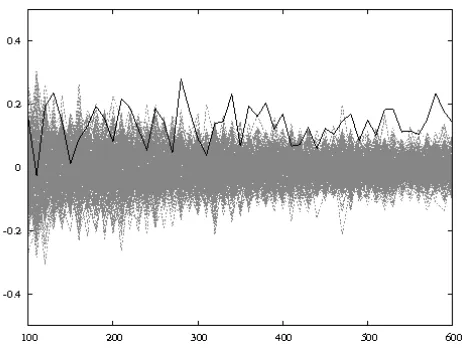
and a confidence level must hence be associated a priori to the choice before the decision is made. Clearly the soundness of the latter process depends on both the selection and the confidence, which must hence be carefully defined. In particular, to be effective in a practical setting, the confidence associated to a decision must be accurately evaluated even for a small number of observations.
This need is illustrated in Figure 1. An usual selection rule is to simply choose the best ranked key. Using 280 observations, this rule would lead to the choice of the right subkey, whereas a wrong subkey would have been chosen using 420 observations. An optimal heuristic would then deem the first attack a success, and the second one a failure.
To evaluate the confidence, we follow a similar approach as in [2] and [9], and we consider the rank of a key and the success rate of an attack as random vari-ables depending on the number of observations. We therefore study thesampling
distribution of these variables, that is, their distribution when derived from a
random sample of finite size.
As an illustration of the sampling distribution of the rank, we run an exper-iment where several CPA targeting the output of the AES sbox are performed, assuming a Hamming weight leakage model with a Gaussian noise of standard deviation 3. A random subkeyk0 is drawn, andN leakage observations are
gen-erated. Then, the rankrk,N of each hypothesiskis computed. This experiment
is repeated several times with new leakage observations, and the mean and vari-ance of the associated random variables Rk,N are computed. We then perform
the same experiment on a leakage of standard deviation 10. The results can be seen in Figure 2.
0 50 100 150 200 250
1 10 100 1000 10000
(a)
0 50 100 150 200 250
1 10 100 1000 10000
(b)
0 1000 2000 3000 4000 5000 6000
1 10 100 1000 10000
(c)
0 1000 2000 3000 4000 5000 6000
1 10 100 1000 10000
(d)
Interestingly, the repetition of this process using a different correct keyk00 results in the exact same curves, but none of them is associated with the same hypothesis. In fact, the distribution ofRk,N does not depend on the value of the
hypothesis k, but on its (bit-wise) difference to the correct key k0. As already
mentioned in [9], this can be formally argued by observing that the difference k⊕k0can be rewritten as (k⊕k0⊕k00)⊕k00. Experiments also show that the rate
of convergence is substantially higher for the correct hypothesis, and that the variance of the correct key rank decreases faster than the variance of any wrong key rank. Moreover, the increase of the noise standard deviation only impacts the number of measurements required to observe these patterns.
Figure 2 also hints that the evolution of the sampling distribution of every Rk is eventually related to the value of the correct key and hence brings
in-formation about it. In other terms, the full vector of ranks gives inin-formation on the correct key (and not only the hypothesis ranked first). Based on this observation, it seems natural to use this information to increase the attack effi-ciency and/or the confidence in the attack results. To be able to precisely assess both kinds of increase, the distributions of all the variablesRk therefore need to
be understood. Bearing this in mind, we now formalize some information that an adversary can obtain while performing a side-channel attack on a set L of N independent observations. Scores are computed using aprogressive approach,
i.e.taking an increasing number of traces into account. Namely, the scores are computed after N1 < N observations, then again after N2 > N1 observations,
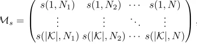
and so on until the N observations inL have been considered. This approach enables the computation of the matrix:
Ms=
s(1, N1) s(1, N2) · · · s(1, N)
..
. ... . .. ... s(|K|, N1)s(|K|, N2)· · · s(|K|, N)
,
where s(k, Ni) denotes the score of the hypothesis k computed usingNi
obser-vations.
According to the Neyman-Pearson lemma [8], an optimal selection rule would then require the knowledge of the statistical distribution of this matrix when the correct subkey is known. In a real attack setup however, the latter subkey is unknown and one then has to proceed with a likelihood-ratio approach in order to retrieve it. Even optimal from an effectiveness point of view, this approach is not realistic as it reposes on two major issues: the knowledge of the distribution of the matrix (which requires a theoretical study over highly dimensional data) and the computation and storage of every score (which may require a lot of time and memory). Moreover, one could wonder if all the information contained in the matrix is relevant, or if there is some redundancy. On the opposite side, the actual attacks only use small parts of the available information. For example, the classical selection of the best ranked key simply amounts to choose the maximum of the last column of scores inMs. Between those two extrem approaches, one
Related work The problem of evaluating the success of an attack has already been tackled in several papers [2, 6, 9, 10]. In [6] and [10], the CPA success rate is evaluated by using Fisher’s transformation (see for instance [3]): simple formulae are exhibited to estimate the success rate in terms of both the noise standard deviation and the correlation corresponding to the correct key. These works were a first important step towards answering our problem. However, they are con-ducted under the assumption that wrong hypotheses are uncorrelated to the leakage. As illustrated in Figure 2 (and as already noticed in several papers), this assumption, sometimes calledwrong key randomization hypothesis [5], does not fit with the reality: each hypothesis score indeed actually depends on the bit-wise difference between the hypothesis and the correct key. The error induced by the assumption is not damaging when one only needs to have an idea about the general attack trends. It is however not acceptable when the purpose is to have a precise understanding of the attack success behavior and of the effect of the sbox properties on it. This observation has been the starting point of the analyses conducted in [2] and [9], where the wrong key randomization hypothesis is relaxed. In Rivain’s paper, a new and more accurate success rate evaluation formula is proposed for the CPA. In [2], Feiet al.introduce the notion of
confu-sion coefficient, and use it to precisely express the success rate of the monobit
DPA. This work can be viewed as a specification of Rivain’s, as monobit DPA is a particular case of a CPA [1]. This point is formally stated in Section 2.3.
Several criteria indicating the effectiveness of side-channels have also been studied to compare side-channel attacks (e.g. [11]). Among those, the particular behavior of the right subkey ranking have been exploited in [7] to propose an improvement of the attack efficiency when the correct key is unknown. This approach illustrates the importance of such criteria in practical attacks, but it is purely empirical.
Contributions In this paper, we focus on the estimation of the success of an attack in both contexts of known and unknown correct key. In Section 2, state of the art evaluations of the CPA success rate are compared under the Hamming weight leakage model. In Section 3, the impact of the evolution of ranks on the confidence level is studied, and the success rate is used to give a theoretical ground to these results. Finally, conclusions are drawn and new questions are opened in Section 4.
2
CPA success rate
2.1 Notations
Vectors (resp. matrices) with coordinatesxi(resp.xij) are denoted by (xi)i(resp.
(xij)i,j). Indices bounds are omitted if not needed. For any random variableX,
and varianceσ2, we denote it byX ∼ N(µ, σ2). The set of subkey hypotheses is
denoted byK, andk0∈ Kdenotes the correct key,i.e.the subkey actually used
by the algorithm. We assume thatKis a group for the bit-wise addition and for any δ ∈ K, we denote bykδ the element such thatkδ = k0⊕δ. Furthermore,
we denote by X a (discrete) random variable whose realizations are known to the attacker, by Zδ the random variable associated to the output of a function
f such that Zδ =f(X⊕kδ), and by L the random variable associated to the
leakage on Z0. For any i, we denote byxi andli the i-th realization of X and
L, and by zδ,i thei-th realization ofZδ. For a fixed numberN of observations,
we denote byρδ the Pearson correlation coefficient between (l1, l2,· · ·, lN) and
(zδ,1, zδ,2,· · ·, zδ,N). Eventually, we denote the rank ofkδbyRδ. By definition, it
is equal to the number of hypotheseskδ0 such thatρδ0 > ρδ. We will sometimes
use the notationρδ(N) andRδ(N) to reveal the functional dependency between
ρδ (respectively Rδ) andN.
2.2 Theoretical success rate
In this section we aim to compare the theoretical evaluations of the CPA suc-cess rate given by [6], [10] and [9]. We recall that, according to the introduced notations, the success rateSR of an attack satisfies:
SR=P(R0(N) = 1), (1)
or equivalently
SR=P(ρ0(N)−ρ1(N)>0,· · ·, ρ0(N)−ρ|K|−1(N)>0). (2)
Mangard’s study in [6] is conducted in the particular case where |K| = 2 (i.e.when there are only two subkey candidates to test). It is moreover based on the three following assumptions:
Assumption 1 [Input uniformity]The input random variable X is uniformly distributed.
Assumption 2 [Gaussian distribution of the leakage]Thei-th leakage satisfies
li=f(xi⊕k0)+βi, whereβiis the realization of an independent random variable
B∼ N(0, σ2), andf is a known function.
Remark 1. Usually, f is of the form ϕ◦S, where ϕ is surjective and S is a
balanced function.
Assumption 3 [Nullity of the wrong hypotheses’ correlation coefficients] The correlation coefficient corresponding to a wrong hypothesis is asymptotically null.
Using Fisher’s Z-transformation, the following approximation of (1) is then obtained:
SR'
Z ∞
0
1
1
√
N−3
√
2πexp−
(x−√ 1 1+σ2)
2
2
N−3
dx
!
The latter approximation has been further extended to any subkey set of size
|K|by Standaertet al.in [10]:
SR'
Z ∞
0
1
1
√
N−3
√
2πexp−
(x−√ 1 1+σ2)
2
2
N−3
dx
!|K|−1
. (4)
In subsequent works, Rivain [9] and Feiet al. [2] have argued that Assump-tion 3 is usually not satisfied, which induces an error (possibly high) in (3) and (4) approximations. This observation led Rivain to conduct a new theoretical study of the success rate where the latter assumption is relaxed, and Assump-tion 1 is replaced by the following one:
Assumption 1 bis [Equality of the inputs occurrences] Every possible value
x∈ X occurs the same number of times in the sample used for the attack.
Remark 2. This assumption implicitly considers that the study is done by fixing
the values taken byX (which is hence no longer a random variable).
Remark 3. When the plaintexts used in the attack are generated uniformly at
random and if their number is reasonably high, then the occurrences of every possible valuexare very likely to be close to each other.
Under Assumption 1 bis, Rivain has shown that the distribution of the scores vector (ρ0(N), ρ1(N),· · · , ρ|K|−1(N)) produces the same ranking as a new vector
d(N) called the distinguishing vector and defined such that
d(N) = (Γ0(N), Γ1(N),· · ·, Γ|K|−1(N)), where Γδ(N) is the random variable
associated to the sum N1 PNi=1zδ,ili. It is also observed that evaluating the rank
Rδ(N) of a key hypothesiskδ (at a differenceδ of the correct keyk0) amounts
to study the number of positive coordinates in the (|K| −1)-dimensional
com-parison vectorcδ(N) = (Γδ(N)−Γ0(N),· · ·Γδ(N)−Γ|K|−1(N)) (i.e.the vector
obtained by subtracting d(N) to (Γδ(N),· · ·, Γδ(N)), followed by the deletion
of theδ-th coordinate). Thanks to this rewriting of the CPA success rate estima-tion in terms ofd(N) andcδ(N), and considering an independent noise, Rivain
proves the two following theorems1:
Theorem 1. [9] In a CPA exploitingN observations leakages, the
distinguish-ing vector d(N)follows a multivariate normal distributionN(µd, Σd(N)), such
that:
µd= (κ0, κ1,· · · , κ|K|−1),
whereκδ =|X |1 Px∈Xzx,0zx,δ and
Σd(N) =
σ2
N(κi⊕j)0≤i,j≤|K|−1
1
Theorem 2. [9] In a CPA exploitingN observation leakages, the comparison
vectorcδ(N)follows a multivariate normal distributionN(µδ, Σδ(N)), such that:
µδ = (κδ−κi)i6=δ
and
Σδ(N) =
σ2
N(κ0−κi−κj+κi⊕j)i,j6=δ.
These theorems allow to accurately deduce the distribution of the vectors
d(N) andcδ(N), from the noise varianceσ2and a modeling ofϕ. They therefore
permit the computation of the probability P(Rδ(N) = 1) for any δ (i.e. the
probability that the hypothesis at differenceδof the correct key is ranked first). According to (1), it may consequently be applied to compute the CPA success rate, which leads to the following success rate evaluation2:
SR=Φ|K|−1(µ0, Σ0(N)), (5)
whereΦ|K|−1 denotes the cdf of the (|K| −1)-dimensional normal distribution of
parameters µ0 and Σ0. In Section 2.3, this new approximation is compared to
(4) and it is indeed shown to be more precise.
The coefficient κi in Theorems 1 and 2 can be seen as an extension of the
definition of theconfusion coefficient introduced by Feiet al. in [2] to estimate the efficiency of a monobit DPA. By analogy with [2], we hence propose the following definition:
Definition 1 (CPA confusion coefficient). Let k0 be the correct hypothesis
and kδ be an element of K, for x ∈ X, let zx,0 and zx,δ be defined such that
zx,0=f(x⊕k0)andzx,δ=f(x⊕kδ)for some functionf. The CPA confusion
coefficientκδ is then defined by3:
κδ =
1
|X |
X
x∈X
zx,0zx,δ.
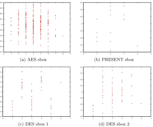
In Figure 3, we illustrate the CPA confusion coefficient in the case wheref is the composition of the Hamming weight with some classical sbox. Moreover, Definition 1 implies that, similarly to the expression of the success rate of the DPA proposed in [2], the formula for the CPA success rate can be related to confusion coefficients capturing the impact of the algebraic properties of the cryptographic primitive on the attack efficiency.
In the following section, we compare the formulae of [10] and [9] against experimental simulations of CPA on AES.
2
This estimation supposes that the covariance matrixΣ0(N) is not singular. When
Σ0(N) is singular, other numerical evaluations can be performed (e.g. [4]). In both
cases, empirical evaluations ofSRcan be performed by simulating random vectors d(N) orc0(N) following respectivelyN(µd, Σd(N)) orN(µ0, Σ0(N)).
3
15.5 15.6 15.7 15.8 15.9 16 16.1 16.2 16.3 16.4
0 1 2 3 4 5 6 7 8 9
(a) AES sbox
3.2 3.4 3.6 3.8 4 4.2 4.4 4.6
0 1 2 3 4 5
(b) PRESENT sbox
3.5 3.6 3.7 3.8 3.9 4 4.1 4.2 4.3 4.4 4.5
0 1 2 3 4 5 6 7
(c) DES sbox 1
3.6 3.7 3.8 3.9 4 4.1 4.2 4.3 4.4
0 1 2 3 4 5 6 7
(d) DES sbox 2
Fig. 3.Values ofκδunder the assumption thatϕis the Hamming weight function, for
different sboxesS, in function of the Hamming weight ofδ.
2.3 Comparison on AES
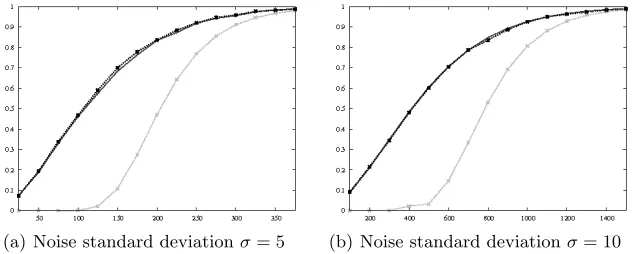
In the following, we suppose that the function S is the AES sbox, and that the functionϕ is the Hamming weight function. First, we estimate the success rate of a CPA empirically, by performing several thousands of attacks. Then, we evaluate Formula (4). Finally, we compute all confusion coefficients, deducing µ0andΣ0(N), and we estimate the success rate by evaluating Formula (5). The
results are plotted in Figure 4. Formula (5) matches the empirical results quite well. This is mainly due to the relaxing of Assumption 3.
3
Confidence in a result
When performing an attack without the knowledge of the correct subkey k0,
the adversary needs to determinehow to select the most likely hypothesis, and
(a) Noise standard deviationσ= 5 (b) Noise standard deviationσ= 10
Fig. 4.Evaluations of the CPA success rate in function of the number of measurements, according to either empirical results (plain black), Formula (4) (dashed light grey) and Formula (5) (dashed dark grey).
several CPA using an increasing number N of observations and we compute the attack success rate as a function ofN. In the second case, we perform the same CPA but we output a candidate subkey only if it has been ranked first both withN and N2 observations. For the latter experiment, we plot the attack success rate considering either the total number of experiments in dotted light grey and considering only the experiments where a key candidate was output (i.e.appeared ranked first withN and N2 observations) in dashed light grey.
As it can be seen on Figure 5, the attack based on the stabilization criterion has a better chance (up to 15%) to output a correct result if it outputs anything. However, its overall success rate is significantly lower than the classical CPA success rate. The candidate selection rule hence increases the confidencein the selected subkey but decreases the success rate. In fact, we argue here that the two notions are important when studying an attack effectiveness. When attacking several subkeys separately, the assessment of a wrong candidate as a subpart of the whole secret key will lead to an indubitable failure, whereas a subkey that is not found (because the corresponding partial attack does not give a satisfying confidence level) will be bruteforced.
In the following, we give a theoretical justification to this empirical and natural attack effectiveness improvement. To this end, we introduce the notion
ofconfidence, which aims at helping the adversary to assess the success or failure
of an attack with a known error margin.
3.1 Confidence in an hypothesis
Applying the notations introduced in Section 1, we assume that a partial attack is performed on a set of N independent observations and aims at the recovery of a correct subkeyk0 among a set of hypotheses. For our analysis, the score of
0 0.1 0.2 0.3 0.4 0.5 0.6 0.7 0.8 0.9 1
50 100 150 200 250 300 350
(a) Noise standard deviationσ= 5
0 0.1 0.2 0.3 0.4 0.5 0.6 0.7 0.8 0.9 1
200 400 600 800 1000 1200 1400
(b) Noise standard deviationσ= 10
Fig. 5.Evaluations of the correctness of the output of attacks in function of the number of observationsN in different contexts: 1) the best ranked subkey is always returned (plain dark grey, 2)) the best ranked subkey is returned only when it was also ranked first with N2 observations and the success is computed against the number of times both attacks returned the same result (dashed light grey) 3) the best ranked subkey is returned only when it was also ranked first with N2 observations and the success is computed against the number of times the attack has been launched (dotted light grey).
then again afterN2 > N1 observations, and so on until theN observations are
considered. In the sequel, the attack onNi observations is called thei-th attack.
All those attacks result in a matrixMscontaining the scoress(k, Ni) for every
hypothesiskand every number Ni of observations. With this construction, the
last column vector (s(k, N))k corresponds to the final attack scores, whereas
(s(k, Ni))k corresponds to intermediate scores (for the i-th attack). In other
terms, the right-column of Ms is the attack result, and the rest of the matrix
corresponds to the attack history. With this formalism in hand, the key candidate selection may be viewed as the application of some selection rule R to Ms,
returning a subkey candidate KR. The question raised in the preamble of this section may then be rephrased as: ”For some ruleR, what is the confidence one can have inKR ?”. To answer this question, we introduce hereafter the notion
ofconfidence inKR.
Definition 2 (Confidence). For an attack aiming at the recovery of a keyk0
and applying a selection ruleRto output a candidate subkeyKR, the confidence
is defined by:
c(KR) = P(K
R=k
0)
P
k∈KP(KR =k)
.
Remark 4. Theconfidence level associated to a rule Rmerges with the notion
Let us illustrate the application of the confidence level with the comparison of the two following rules, corresponding to the criterion described in the preamble of this section:
– RuleR0: output the candidate ranked first at the end of theN−thattack.
– RuleRt: output the candidate ranked first at the end of theN−thattack,
only if it was also ranked first for all attacks performed using Nt to N
observations.
By definition of R0, and using the notations of Section 2, the confidence
associated to R0 satisfies:
c(KR0) = P(R0(N) = 1)
P
δP(Rδ(N) = 1)
=P(R0(N) = 1),
which can be computed thanks to Theorem 2. With a similar reasoning, we have:
c(KRt) =P(R0(Nt) = 1, R0(Nt+1) = 1,· · ·, R0(N) = 1) P
δP(Rδ(Nt) = 1, ,· · ·, Rδ(N) = 1)
,
whose evaluation requires more development than that of c(KR0). For such a purpose, the distribution of the ranks vector (Rδ(Nt), Rδ(Nt+1),· · ·, Rδ(N))
needs to be studied4. We thus follow a similar approach as in Section 2, and we
build theprogressive comparison vectorcδ,t(N) = (cδ(Nt)||cδ(Nt+1)|| · · · ||cδ(N))
where||denotes the vector concatenation operator. We then apply the following proposition, whose proof is given in Annex A:
Proposition 1. For a CPA exploiting a number N of observations, the
pro-gressive comparison vector cδ,t(N) follows a multivariate normal distribution
N(µδ,t, Σδ,t(N)), whereµδ,t is a|K|(N−Nt)vector andΣδ,t is a|K|(N−Nt)×
|K|(N−Nt)matrix, satisfying:
µδ,t= (κδ−κ0,· · · , κδ−κ|K|−1, κδ−κ0,· · ·, κδ−κ|K|−1),
and
Σδ,t(N) =
N
max(i, j)Σδ
Nt≤i,j≤N
Proposition 1 allows for the evaluation of the distribution of cδ,t(N), and
thus for the evaluation ofP(Rδ(Nt) = 1, Rδ(Nt+1) = 1,· · · , Rδ(N) = 1) for all
hypotheseskδ. We are then able to compute the confidencec(KRt).
As an illustration, we study the case where a single intermediate ranking is taken into account,i.e.we study the probabilityP(Rδ(N2) = 1, Rδ(N) = 1), and
we plot in Figure 6 the obtained confidences.
As we can see, the confidence estimation matches the empirical results of Figure 5. At any number of observations, the rule Rt actually increases the
confidence in the output of an attack compared to the ruleR0.
4
It is worth noting at this point that the variableRδ(Ni) does not verify the Markov
Fig. 6.Evaluation of confidences in function of the number of measurements for R0
(plain dark grey), and forRN
2 (dashed light grey), withσ= 10.
3.2 Discussion and empirical study of convergence rules
The accurate evaluation of the confidence level allows a side-channel attacker to assess the success or failure of a partial attack with a known margin of error. For example, and as illustrated in previous section, applying the selection rule
R0 for a CPA on 800 noisy observations (with noise standard deviation equal
to 10) leads to an attack failure in 18% of the cases. As a consequence, to reach a 90% confidence level, the attacker has either to perform the attack on more observations (1000 in our example), or to use an other selection rule. Indeed, different selection rules lead to different confidence levels, as they are based on different information. Though a rule based on the whole matrix Ms would
theoretically give the best results, the estimation of the confidence level in such a case would prove to be difficult. An interesting open problem is to find an acceptable tradeoff between the computation of the involved probabilities and the accuracy of the obtained confidence.
In this section, we study a new rule exploiting theconvergence of the best hypothesis’ rank, echoing the observation made in Section 1. To this end, we consider a rule Rγt (with 1 ≤ γ ≤ |K|) and define it as a slight variation of
Rt. The rule R γ
t returns the best ranked key candidate after the N-th attack
only if it was ranked lower than γ for the attack on Nt observations. As in
previous section, we simulate the simple case where only the ranking obtained with an arbitrary number x of observations is taken into account. We hence experimentally estimate the confidence given byRγ
xfor allγ in Figure 7.
For example, when the final best ranked key is ranked lower than 50 using 200 messages, the confidence is around 94% (compared to 92% when usingR0).
100 200 300 400 500 600 700 800 900 1000 0
50 100 150 200 250
0.93 0.935 0.94 0.945 0.95 0.955 0.96 0.965 0.97
Fig. 7. Confidence in the key ranked first after a CPA on 1000 observations with σ = 10, knowing that it was ranked below a given rank γ (in y-axis) on a smaller number of measurementsNt (inx-axis).
4
Conclusion
Results presented in this paper are twofold. We first compared several state of the art theoretical evaluations for the success rate of the CPA, and we linked them with the notion of confusion coefficient, capturing the effect of the cryptographic primitive on the difference between the correct hypothesis and the wrong ones. Secondly, we give a rationale for the use of some empirical criteria (such as the convergence of the best hypothesis’ rank towards 1) as indicators of the attack success. We hence involve the notion of confidence to allow for the accurate estimation of this success.
As an avenue for further research, this work opens the new problem of the exhibition of novel selection rules allowing to efficiently and accurately evaluate the confidence in a side-channel attack while conserving an acceptable success rate.
References
1. J. Doget, E. Prouff, M. Rivain, and F.-X. Standaert. Univariate Side Channel Attacks and Leakage Modeling. Journal of Cryptographic Engineering, 1(2):123– 144, 2011.
2. Y. Fei, Q. Luo, and A. A. Ding. A Statistical Model for DPA with Novel Algorith-mic Confusion Analysis. In E. Prouff and P. Schaumont, editors, CHES, volume 7428 ofLecture Notes in Computer Science, pages 233–250. Springer, 2012. 3. R. A. Fisher. On the mathematical foundations of theoretical statistics.
Philo-sophical Transactions of the Royal Society, 1922.
4. A. Genz and K. shing Kwong. Numerical evaluation of singular multivariate normal distributions. Journal of Statistical Computation and Simulation, 68:1–21, 1999. 5. C. Harpes. Cryptanalysis of iterated block ciphers. InETH Series in Information
Processing, volume 7. Hartung-Gorre Verlag, 1996.
6. S. Mangard. Hardware Countermeasures against DPA – A Statistical Analysis of Their Effectiveness. In T. Okamoto, editor,Topics in Cryptology – CT-RSA 2004, volume 2964 ofLecture Notes in Computer Science, pages 222–235. Springer, 2004. 7. M. Nassar, Y. Souissi, S. Guilley, and J.-L. Danger. ”Rank Correction”: A New Side-Channel Approach for Secret Key Recovery. In M. Joye, D. Mukhopadhyay, and M. Tunstall, editors,InfoSecHiComNet, volume 7011 ofLecture Notes in Com-puter Science, pages 128–143. Springer, 2011.
8. J. Neyman and E. S. Pearson. On the problem of the most efficient tests of statistical hypotheses. Philosophical Transactions of the Royal Society of London. Series A, Containing Papers of a Mathematical or Physical Character, 231:289– 337, 1933.
9. M. Rivain. On the Exact Success Rate of Side Channel Analysis in the Gaussian Model. In R. Avanzi, L. Keliher, and F. Sica, editors,Selected Areas in Cryptog-raphy, Lecture Notes in Computer Science, pages 165–183. Springer, 2008. 10. F.-X. Standaert, E. Peeters, G. Rouvroy, and J.-J. Quisquater. An overview of
power analysis attacks against field programmable gate arrays. IEEE, 94(2):383– 394, 2006.
11. C. Whitnall and E. Oswald. A Comprehensive Evaluation of Mutual Information Analysis Using a Fair Evaluation Framework. In P. Rogaway, editor, CRYPTO, volume 6841 ofLecture Notes in Computer Science, pages 316–334. Springer, 2011.
A
Proof of proposition 1
By its construction, the progressive comparison vector cδ,t(N) follows a
mul-tivariate normal law N(µδ,t, Σδ,t(N)). Its mean vectorµδ,t is trivially deduced
from the expression of µδ given in Section 2. To compute the expression of
Σδ,t(N), we hence only need to prove the following lemma:
Lemma 1. For any hypotheses(i, j, j0)∈[0,|K| −1]3 and for any sets of
obser-vations of sizesNt andN (such that Nt< N), Assumptions 2 and 4 imply:
Cov[Γi(N)−Γj(N), Γi(Nt)−Γj0(Nt)] =
Nt
Proof. By the definitions of Γi(N) and Γj(N), the following equality holds:
Γi(N)−Γj(N) = N1(
PNt
t=1lt(zi,t−zj,t) +
PN
t=Nt+1lt(zi,t−zj,t)). This can be
rewritten asΓi(N)−Γj(N) =N1(Nt(Γi(Nt)−Γj(Nt)) +
PN
t=Nt+1lt(zi,t−zj,t)).
The independence of all observations and the bilinearity of the covariance then
suffice to prove the lemma. ut
The coefficients ofΣδ,t(N) can hence be easily computed, using this Lemma.
B
Confidence gain with the difference of scores
We study a transverse approach to the one described in Section 3, by observing the last vector of scores (instead of the rank obtained from intermediate attacks). Namely, we focus on a rule outputting the best ranked candidate when the difference between its score and the score of every other hypothesis is greater than a certain value. This criterion is considered for example in [11]. We simulate this rule, for several bounds, and we plot the results in Figure 8. It is of particular
100 200 300 400 500 600 700 800 900 1000 0.02
0.04 0.06 0.08 0.1 0.12 0.14 0.16
0.1 0.2 0.3 0.4 0.5 0.6 0.7 0.8 0.9 1
Fig. 8.Confidence in the best ranked key after a CPA withσ= 10, on a given number of observations (inx-axis), knowing that its score is higher by a certain value (in y-axis) than every other hypothesis score.