Handling Noise and Outliers in Single Image
Deblurring using L0 Sparsity
Aparna Ashok
1, Deepa P. L.
2PG Student[Signal Processing] ,Dept. of ECE, Mar Baselios College of Engineering and Technology,
Thriruvananthapuram, Kerala, India1
Assistant Professor, Dept. of ECE, Mar Baselios College of Engineering and Technology, Thiruvananthapuram,
Kerala, India2
ABSTRACT: Camera shake during exposure leads to image blur and poses an important problem in digital photography. Blind deconvolution recovers the sharp original image from a blurred image. MAP has been the most widely used deconvolution field but naive MAP methods mostly tends to favour no-blur solution. An intermediate representation of the image called unnatural representation has been found to the main reason for success of existing MAP based methods. This paper presents a new blind deconvolution algorithm based on L0 sparsity for single image
motion deblurring, which is robust to the presence of noise. Directional filtering is used for noise handling process owing to the fact that it does not interfere with blur of the image affecting the kernel estimation process adversely. Also, a non-blind deconvolution step with explicit outlier handling is incorporated in final image restoration step which ensures that the image is devoid of ringing artifacts and handles other non-linearities. This presents an efficient optimization problem which requires only a few iterations solve and provides very good visual quality images with no ringing artifacts despite the presence of noise. The results are comparable to state-of-the-art methods dealing with images affected with only blur while being robust to noise unlike state-of-the-art methods.
KEYWORDS: Camera shake, motion blur,L0 sparsity, directional filtering, outlier handling, ringing artifacts.
I.INTRODUCTION
sensors, hot pixels etc. These outliers are very common in the imaging process but they are often unaccounted by the existing deconvolution methods. The outliers cause violation of linear blur model which leads to ringing artifacts inspite of the accurate estimation of the motion blur kernel, which is another challenging issue in the deblurring process.
This paper proposes a new blind deconvolution algorithm with L0 sparse prior for recovering the original image from a
blurry and noisy image, which uses directional filtering for noise handling and includes an efficient non-blind deconvolution step equipped with outlier handling which ensures the estimation of a latent image free of ringing artifacts. It has been already pointed out by studies that naive MAP approach fails to give the desired result for natural images and Levin et al.[1] has analyzed the different sources of the failure. The success of the existing MAP based approaches has been found to be due to the intermediate step which produces an image which contains only the salient structures of the image while suppressing others. This intermediate image consists of only high contrast step like structures. The prior MAP based approaches that are successful can be roughly classified into two types i.e. those with explicit edge prediction steps like using a shock filter [2,3,4,5,6,7,8] and those which include implicit regularization process[9,10]. The common factor is the intermediate image consisting of only step like structures called the unnatural representation of the image, which is the key factor in the success of MAP based methods. This unnatural representation is the fundamental step in the image deblurring process using L0 sparse prior and it enables accurate kernel estimation in
comparatively lesser number of iterations. Directional filters are experimentally seen to have the specific property which removes noise in an image effectively, without affecting the blur kernel estimation process in a significant manner. So, directional filtering can be incorporated into the blind deblurring process for noise handling, without the risk of interfering with the kernel estimation process and degrading the final result. The use of a final blind deconvolution process equipped with an explicit model for outlier handling results in a final latent image without ringing artifacts. The pixels of an image can be classified into inlier pixels that satisfy the linear blur model and outlier pixels that violate the same. An expectation maximization (EM) method is employed to refine the outlier classification and the latent image iteratively while removing the possibility of any ringing artifacts in the estimated image.
II.RELATED WORK
Many single image blind deblurring methods have been proposed in the recent years and the field has achieved considerable progress with many milestones. The basic concept of blind deconvolution and different existing types of blind deconvolution algorithms are explained in detail by D. Kundur and D. Hatzinakos in their paper [11]. The classifications of blind deconvolution techniques are explained and its merits and demerits are discussed. MAP method is the most commonly used among the blind deblurring techniques because it does not require any apriori information about the PSF and also, it does not constrain the PSF to be of any specific parametric form. Naive MAP approach was seen to fail on natural images as it tends to favor no blur solution. Levin et al. [1] analyzed the source of MAP failure and demonstrated that marginalizing the process over the image x and MAP estimation of the kernel k alone proves successful and recovers an accurate kernel. As noted by Levin et al. [1] and Fergus et al. [12], blurry images have a lower cost compared to sharp images in MAP approach and as a result blurry images are favored. So, a number of more complex methods have been proposed that include marginalization over all possible images [1,12], dynamic adaptation of the cost function used [13], determining edge positions by the usage of shock filtering [2] and reweighting of image edges during optimization [3]. Many papers emphasized the usage of sparse prior in the derivative domain to favor sharp images. But expected result has not been yielded by the direct application of this principle, as it required additional processes like marginalization across all possible images as demonstrated by Fergus et al. [12] spatially varying terms or solvers that vary optimization energy over time as shown by Shan et al.[13]. Krishnan et al. [9] used l1/l2 norm as the
sparsity measure which acts as a scale invariant regularizer. Xu et al. [10] introduced L0 sparsity as regularization term,
which relies on the intermediate representation of image for its success. Pan et. al. [14] also adopted L0 regularization
better manner compared to the previous methods, using a single threshold value to detect saturated pixels is an erroneous process and fixing an optimal threshold is a complicated problem. Yuan et al. [23] proposed a coarse to fine progressive deconvolution process where bilateral regularization is used to remove ringing artifacts and sharpen the edges of the image at each stage. This is a process which implicitly handles the outliers by directly suppressing the existing artifacts at each step. Cho et al. [24] proposed a much more efficient method for outliers handling which models outlier values in the blur model itself and produces a good results with negligible ringing effects.
III.PROPOSED WORK
The paper bases itself on the observation of experimental facts that the success of the existing MAP based methods is due to the unnatural representation of the image and proposes an L0 approximation scheme as a regularization term
which guides the blur kernel estimation process. The paper deals with blurry and noisy images and aims to obtain a good quality latent image, with negligible ringing artifacts, in spite of the presence of noise. Most of the existing standard deblurring techniques assume ideal conditions with little noise and they produce fairly good results in these conditions. On the other hand, these methods fail to produce satisfactory results in the presence of noise. Even state-of-the-art denoising techniques have an adverse effect on kernel estimation process as they tend to cause information loss, thus resulting in inaccurate kernel estimation and distorted final deblurring result. In this paper, appropriate noise handling is included by means of directional low pass filtering of the images. Directional filtering removes the noise to a high level, but does not run the risk of steering the kernel estimation process in the wrong direction or eventually affecting the kernel estimation process significantly in an adverse manner. Incorporation of a final non-blind deconvolution step, which handles outliers like non-Gaussian noise and saturated pixels efficiently by explicit outlier modeling, helps to render much better quality results with no ringing artifacts.
Directional low pass filters can be applied to an image to reduce its noise level without affecting the process of kernel estimation adversely on a significant level. The application of directional low pass filter 𝜃 to an image I can be explained theoretically by the equation
𝐼 𝑝 ∗ 𝜃 = 1
𝑟 𝑤 𝑡 𝐼(𝑝 + 𝑡𝑢𝜃
∞
−∞ ) 𝑑𝑡 (1)
where p denotes the location of each pixel, , t is the spatial distance from each pixel to p, r is the normalization factor which is given by 𝑟 = −∞∞ 𝑤 𝑡 𝑑𝑡 and 𝑢𝜃 is the unit vector in the direction of application of the directional filter, θ. We assume a Gaussian profile for the directional filter and this is determined by the factor w(t) which can be given by the expression 𝑤 𝑡 = 𝑒−𝑡2/2𝜎2 where σ is the standard deviation term which controls the strength of the Gaussian directional filtering process [25].
A regularization term which consists of a family of loss functions, that approximates L0 cost, is incorporated into the
objective function which has to be optimized for the kernel estimation process. L0 approximation process enables a high
sparsity pursuit regularization, which leads to consistent energy minimization and fast convergence in a fewer number of iterations. Since only the salient structures of the image are retained in its unnatural representation, the method is much faster than other implicit sparse regularization methods. This family of loss functions that approximates L0 cost into the
objective function, implements graduate non-convexity into the optimization process. Consequently, the significant edges present in the intermediate representation swiftly guides the kernel estimation process in the right direction ,thus quickly improving the estimation process in comparatively only a few numbers of iterations.
Saturated pixels: As the camera sensors have a limited dynamic range, pixels receiving more light than the maximum range will be saturated and corresponding pixel intensity values will be clipped. This occurs very commonly in the night shoot scenario with long exposure times as a result of low lighting, where mostly the scene is dark except some very few bright spots which results in saturated pixels. This clipping is a non-linear process which violates the blur model and consequently cause ringing artifacts around these portions.
Non-Gaussian noise: The state-of-the-art deblurring method assumes the noise infecting the image to be Gaussian and hence the deconvolution method assumes a Gaussian noise model. But an image can be affected by various other types of noise too, which cannot be handled by the existing deblurring methods because they assume a specific type of noise model and is not robust enough to handle other cases of noise. These non-Gaussian noise acts as outliers and cause ringing artifacts in the restored image result.
Non-linear camera response: Digital cameras have various processing units, many of which are non-linear. For instance, the radiance of a scene is mapped to pixel intensities using a non-linear response curve. This violates the linear blur model, thus becoming a cause for artifacts. But, this is a type of outlier which is comparatively easier to avoid than the other two. This is possible by taking the raw camera output or by applying the inverse response curve obtained from camera calibration in the pre-processing stage.
Although these outliers vary in nature, they basically cause the same impacts to the deconvolution process. They cause the linear blur model to fail and they cause the noise to be non-Gaussian. We propose a non-blind deconvolution step that specifically handles these two violations by explicit outlier modeling and handling.
IV.MATHEMATICAL FRAMEWORK
We denote the latent image by 𝑥, blurred and noisy image by 𝑦 and the blur kernel by 𝑘 . The blurring process can be represented generally by the expression
𝑦 = 𝑘 ∗ 𝑥 + 𝜂 (2)
where η represents the image noise. The blurred and noisy image𝑦is initially denoised by the application of directional low pass filters with Gaussian profile in the desired orientations. The strength of the filtering process by directional filter
𝜃along each orientation θ is denoted by its σ value. This value can be decided accordingly based on the noise infected image and the density of the noise along that particular direction. After deciding on the different orientations for the application of directional filters and the σ value along each orientation that decides the strength of Gaussian profile filtering along that direction, denoising is carried out. This gives a noise-free image without affecting the blur of the image considerably. The denoising process carried out does not interfere with accurate kernel estimation or steer the estimation process in wrong direction.
The framework of the proposed deblurring technique includes a loss function Ф0(.) that approximates L0 cost into the
objective function that has to be optimized . Loss function Ф0(.) for an arbitrary image z can be defined as
Ф0 ∂∗z = Ф 𝜕∗𝑧𝑖 i
(3)
where
Ф 𝜕∗𝑧𝑖 = 1 𝜀2 𝜕∗𝑧𝑖 2
1 ′
𝑖𝑓 𝜕∗𝑧𝑖 ≤ 𝜀
𝑜𝑡𝑒𝑟𝑤𝑖𝑠𝑒 (4) and ∗ 𝜖 {, 𝑣} denoting the horizontal and vertical directions respectively for each pixel 𝑖 of the image. The loss function regularizes the high frequency components of the image by acting upon the gradient vector 𝜕∗𝑧𝑖 for each pixel
𝑖. This is a piecewise function which is continuous when 𝜕 ∗ 𝑧𝑖 ≤ 𝜀, which forms a necessary condition for it to be a loss function mathematically. Ф0(.) is a very high sparsity pursuit function, that approximates sparse L0 function very
Loss function Ф0(.) is incorporated into the final objective function for optimization and it acts as a regularization
term, which in turn guides the kernel estimation in the right direction, by seeking an intermediate representation of the image containing only the salient edges. The objective function for kernel estimation can be given as
𝑚𝑖𝑛
(𝑥 , 𝑘) 𝑘 ∗ 𝑥 − 𝑦 2 + 𝜆 Ф0 ∂∗𝑥
∗∈{,𝑣}
+ 𝛾 𝑘 2} (5)
where 𝑥 is the unnatural representation of the image during the process of optimization of the objective function and
𝜆, 𝛾 are regularization weights . First term in the objective function is the data fidelity term which enforces the blur model constraint, the second term is the loss function which approximates L0 cost into the function and produces
unnatural representation of the image, the third term aids in reducing the noise in the kernel during estimation process. The new regularization term is the key factor in guiding the kernel estimation process in the right direction and results in an accurate estimation of the kernel quickly in a few number of iterations. Using L0 sparse function as regularization term
has an advantage over the usual explicit edge prediction methods used in existing deblurring methods. In the case of explicit edge prediction methods like shock filter implementation or bilateral filtering, it is employed as an additional step and cannot be incorporated into the overall objective function for consistent energy minimization. But the L0 sparse
regularization term can be very efficiently incorporated into the objective function during optimization. This property ensures the fact that the intermediate unnatural representation of the image contains only necessary strong edges that satisfy the constraints, regardless of the blur kernel degrading the image.
The objective function can be solved by alternatively computing the intermediate image value and the kernel value during each iteration [26] . The computation process for (t+1)th iteration of optimization process can be given by Eq. 6 and Eq. 7.
𝑥𝑡+1= 𝑎𝑟𝑔𝑚𝑖𝑛
𝑥 𝑘
𝑡∗ 𝑥 − 𝑦 2+ 𝜆 Ф 0 ∂∗𝑥 ∗∈ ,𝑣
(6)
𝑘𝑡+1= 𝑎𝑟𝑔𝑚𝑖𝑛
𝑘 𝑥
𝑡+1∗ 𝑘 − 𝑦 2+ 𝛾 𝑘 2 (7)
Equation 4 for the loss function can be rewritten as follows with ε as a parameter, for the ease of the optimization process.
Ф 𝜕∗𝑧𝑖 , 𝜀 =
𝑚𝑖𝑛 𝑙∗𝑖
𝑙∗𝑖 0+
1
𝜀2 𝜕∗𝑧𝑖 − 𝑙∗𝑖 2 (8)
where ∗ 𝜖 { , 𝑣} and
𝑙∗𝑖= 𝜕0 ∗𝑥 𝑖
, 𝜕∗𝑥 𝑖 ≤ 𝜀
, 𝑜𝑡𝑒𝑟𝑤𝑖𝑠𝑒 (9)
Equation 8 can be proved to be mathematically equivalent to Eq. 4 .So Eq. 8 can be used to represent the loss function henceforth in the kernel estimation algorithm, for ease of computation and implementation purposes. A family of loss functions are obtained based on this equation by setting the value of ε differently. Fig. 1 shows the family of loss functions for different values of ε starting from 1 to 1/8. It can be seen that the value approaches L0 function further as
the value of ε keeps on decreasing from 1 to 1/8. Equation 6 for the optimization process computing 𝑥 can also be rewritten accordingly based on Eq.8 and Eq.9 .
𝑚𝑖𝑛 𝑥 , 𝑙
1
𝜆 𝑘 ∗ 𝑥 − 𝑦
2+ { 𝑖 ∗𝜖{,𝑣}
𝑙∗𝑖 0+
1
𝜀2 𝜕∗𝑥 𝑖 − 𝑙∗𝑖 2} (10)
𝑥𝑡+1= 𝐹−1 𝐹 𝑘 𝑡
. 𝐹 𝑦 +𝜆
𝜀2 𝐹 𝜕 . 𝐹 𝑙 + 𝐹 𝜕 . 𝐹(𝑙𝑣 𝑣)
𝐹 𝑘𝑡
. 𝐹 𝑘𝑡 + 𝜆
𝜀2 𝐹(𝜕) 2+ 𝐹(𝜕𝑣) 2
(11)
𝑘𝑡+1= 𝐹−1 𝐹 𝑥 𝑡+1 . 𝐹(𝑦)
𝐹 𝑥 𝑡+1 2+ 𝛾 (12)
where F(.) and F(.) are the FFT operator and its conjugate respectively, F-1 is the inverse FFT operation whereas and are vectors concatenating and values for each pixel. Multiplication and division operations are performed in an element wise manner on the complex vectors.
Fig. 1: Plots of the loss function approximating L0 for different values of ε
During the implementation process, we use a family of 4 loss functions with ε ϵ{1,1/2,1/4,1/8}. We start from ε = 1 and then proceed to the other values as illustrated in Figure 1. The number of iterations for different loss functions is set to be inversely proportional to the corresponding value of ε controlling the loss function. This is because of the fact that large ε values cause the loss function approximating L0 cost to be more convex like and hence makes it easier to optimize. So it
requires only a few iterations for the optimization process to complete. The results obtained here is taken as an initialization for further refinement in loss functions with smaller ε values, as they are of more concave nature and difficult to optimize. Also, the blur kernel estimation process is carried out in a pyramid-like fashion, by convention. Kernels are estimated in a coarse to fine manner in an image pyramid. The estimate obtained in one image pyramid level is taken as the initialization for the next level. The optimization process in the t+1th iteration in its finest level is as explained by the equations Eq.11 and Eq.12 . Computation process is similar in the coarser level for different iterations.
The algorithm for kernel estimation process in one image level can be given as follows
Algorithm 1
Input: Blurry and noisy image y
Output: Blur kernel k, deblurred image 𝒙
1 Apply N directional filters to the input image y, where each filter has a direction given by θ=(i.Π/N) i=1,2,...N and N is the number of directional filters. Choose the σ value for each direction accordingly depending on the image.
2 Initialize k from the kernel estimate of coarser scale 3 for t= 1:5
4 //update image 5 ε 1 6 for i=1:4
8 solve for l using Eq.9 9 solve for 𝒙 using Eq.11
10 end 11 ε ε/2
12 end
13 //update kernel 14 solve for k using Eq.12
15 end
The image obtained at the end of kernel estimation step is not the final latent image because it contains only high contrast structures and lacks details. So a non-blind deconvolution step has to be carried out using the obtained kernel and the denoised image. There are many existing non-blind deconvolution steps that can be used including most common ones like using a hyper-Laplacian prior. But we can see that even if the kernel estimated is accurate, the final image obtained after deconvolution is very much affected by ringing artifacts. This is due to the presence of outliers that violates the linear blur model followed by standard algorithms. We go for a method that explicitly models and handles the outliers[19]. Since linear blur model cannot model the outliers, a more accurate blur model has to be proposed. We assume that a noise free image is captured by sensors, it is clipped in such a way that the intensities remain within the dynamic range followed by the addition of noise and outliers within the dynamic range. It can be represented as
𝑦′ = 𝑐 𝑘 ∗ 𝑢 + 𝑛 (13)
where 𝑦′ is the denoised image obtained after directional filtering, u is the latent image, 𝑘 is the estimated kernel, 𝑐 is the clipping function such that 𝑐(𝑢) = 𝑢 if u is within the dynamic range and 𝑐(𝑢) is equal to the maximum or minimum intensity if u is outside the dynamic range. Additive noise n follows a Gaussian distribution for inliers and it can take any arbitary value independent of 𝑘 and 𝑦 ′. We assume a random distribution without any priors for outliers. For classification process, we introduce a binary mapping m such that 𝑚 𝑥 = 1 if the image intensity 𝑦𝑥 is an inlier and
𝑚 𝑥=0 if the pixel intensity 𝑦𝑥 is an outlier where 𝑥 denotes the subscript for pixel index. The problem of finding the most probable latent image can be mathematically modeled by MAP estimation as
𝑢𝑀𝐴𝑃 =
𝑎𝑟𝑔𝑚𝑎𝑥
𝑢 𝑝 𝑢 𝑘, 𝑦′
=𝑎𝑟𝑔𝑚𝑎𝑥
𝑢 𝑝 𝑦′ 𝑘, 𝑢 𝑝(𝑢)
=𝑎𝑟𝑔𝑚𝑎𝑥
𝑢 𝑝 𝑦′, 𝑚 𝑘, 𝑢 𝑝(𝑢)
𝑚 ∈𝑀
= 𝑎𝑟𝑔𝑚𝑎𝑥
𝑢 𝑝 𝑦
′ 𝑚, 𝑘, 𝑢 𝑝 𝑚 𝑘, 𝑢 𝑝(𝑢) 𝑚 ∈𝑀
(14)
where M is the space of all possible configurations of m. Prior p(u) for latent image is given by
𝑝 𝑢 = exp −𝜆𝑔 𝑢 /𝑍𝑝 (15)
where Zp is the normalization constant and
𝑔 𝑢 = {|(∇hu)|α
𝑥 + |(∇vu)|α} (16)
𝑝 𝑦′ 𝑚, 𝑘, 𝑢 = 𝑝(𝑦′𝑥|𝑚, 𝑘, 𝑢)
𝑥
(17)
𝑝 𝑦′
𝑥 𝑚, 𝑘, 𝑢 =
𝑁 𝑦′ 𝑓
𝑥, 𝜎 𝑖𝑓 𝑚𝑥= 0
𝐶 𝑖𝑓 𝑚𝑥 = 1 (18)
where𝑓𝑥 = 𝑘 ∗ 𝑢 and C is the constant denoting the inverse of dynamic range of intensities. Binary mapping variable 𝑚 can also be assumed to be spatially independent. So the classification prior can be written as
𝑝 𝑚 𝑘, 𝑢 = 𝑝(𝑚𝑥|𝑘, 𝑢) 𝑥
= 𝑝(𝑚𝑥|𝑓𝑥) 𝑥
(19)
Probability 𝑝 𝑚𝑥 𝑓𝑥 can be further defined as
𝑝 𝑚𝑥 = 1 𝑓𝑥 = 𝑃𝑖𝑛, 𝑖𝑓 𝑓0, 𝑜𝑡𝑒𝑟𝑤𝑖𝑠𝑒𝑥 ∈ 𝐷𝑅 (20)
where DR is the dynamic range of intensities and Pin is the probability value that denotes the probability of 𝑦′𝑥 being an inlier if it lies within the dynamic range. If 𝑦′
𝑥 is outside the dynamic range, then it is an outlier in any case and so the value of 𝑚𝑥 is definitely 0.
Expectation Maximization (EM) method is used find the optimal latent image 𝑢. EM method evaluates the value of expectation of 𝑝 𝑦′, 𝑚 𝑘, 𝑢 and utilizes this value for finding the value of optimal u by maximizing the posterior probability function 𝑝 𝑢 𝑦′, 𝑚, 𝑘 𝛼 𝑝 𝑦′, 𝑚 𝑘, 𝑢 𝑝(𝑢). The expectation value of 𝑝 𝑦′, 𝑚 𝑘, 𝑢 and optimal u value are calculated alternatively by the E and M step respectively. Expectation value R(u,u0)based on the current estimate u0 is given by the E step of EM method as follows.
𝑅 𝑢, 𝑢0 = 𝐸 [𝑝 𝑦′, 𝑚 𝑘, 𝑢 ]
= 𝐸 [𝑝 𝑦′, 𝑚 𝑘, 𝑢 + log 𝑝(𝑚|𝑘, 𝑢)] (21)
We use the result of deconvolution of denoised image 𝑦′ with a simple Gaussian prior by setting all weights to oneas the initial estimate 𝑢0 , to start with the process. Substituting equations Eq.18 and Eq.20 in the obtained expression of Eq.21, we get the expectation value as
𝑅 𝑢, 𝑢0 = 𝐸 𝑚 𝑥 𝑥
𝑙𝑜𝑔 𝑁(𝑦′
𝑥|𝑓𝑥, 𝜎)
= − 𝐸 𝑚𝑥 2𝜎2 𝑥
𝑦′ 𝑥− 𝑓𝑥
2
22
where 𝐸[𝑚𝑥] is given by
𝐸 𝑚𝑥 = 𝑝(𝑚𝑥= 1|𝑦′, 𝑘, 𝑢0)
= 𝑝 𝑦
′
𝑥 𝑚𝑥, 𝑘, 𝑢0 𝑝(𝑚𝑥|𝑘, 𝑢0)
𝑝 𝑦′ 𝑥 𝑘, 𝑢0
(23)
𝐸 𝑚𝑥 =
𝑁 𝑦′
𝑥 𝑓𝑥0, 𝜎 𝑃𝑖𝑛
𝑁 𝑦′
𝑥 𝑓𝑥0, 𝜎 𝑃𝑖𝑛 + 𝐶 1 − 𝑃𝑖𝑛
, 𝑖𝑓 𝑓𝑥0∈ 𝐷𝑅
0 , 𝑜𝑡𝑒𝑟𝑤𝑖𝑠𝑒
(24)
where 𝑓𝑥0= 𝑘 ∗ 𝑢0. Practically, E[𝑚𝑥] is the only value to be computed at the E step because it determines the
expectation value 𝑅 𝑢, 𝑢0 as a function of latent image 𝑢.
Now, we go for the M step of EM maximization process which computes the optimal latent image 𝑢. M step calculates the estimate 𝑢𝑛 during each revision as
𝑢𝑛=𝑎𝑟𝑔𝑚𝑎𝑥
𝑢 𝑅 𝑢, 𝑢
0 + log(𝑝 𝑢 (25)
This can be rewritten as
𝑢𝑛 = 𝑎𝑟𝑔𝑚𝑖𝑛
𝑢 𝑤𝑥
𝑚|𝑦′
𝑥− (𝑘 ∗ 𝑢)𝑥|2+ 𝛽𝑔 𝑢 (26)
where 𝑤𝑥𝑚 = 𝐸 𝑚𝑥 /2𝜎2. Eq.26 can be minimized by using IRLS algorithm and for that, pixel weights 𝑤𝑥 = |∇hu|𝛼 −2 and 𝑤𝑥𝑣= |∇vu|𝛼 −2 are introduced. The minimization process of Eq.26 can be approximated as
𝑢𝑛= 𝑎𝑟𝑔𝑚𝑖𝑛 𝑢 𝑤𝑥
𝑚|𝑦′
𝑥− (𝑘 ∗ 𝑢)𝑥|
2+ 𝛽𝜑 𝑢 (27)
where
𝜑 𝑢 = {𝑤𝑥 𝑥|(∇hu)x|2+ 𝑤𝑥𝑣 (∇vu)x|2 (28)
Eq.28 becomes a quadratic function with respect to 𝑢 for fixed values of 𝑤𝑥 and 𝑤𝑥𝑣 and it can be solved by conjugate gradient method. Minimization operation defined in Eq.26 can be achieved by alternating between updating the values of
𝑤𝑥 and 𝑤𝑥𝑣 and minimizing Eq. 27.The theoretical aspect of EM minimization can be explained by considering the meaning behind the expression 𝐸[𝑚𝑥].If pixel intensity 𝑦′𝑥is an inlier, the expectation value computed in E step is close to unity. In the M step that follows, only inliers with large weights are used as pixel weights in the deconvolution process whereas outliers with lower weights from E step are excluded from the deconvolution process for obtaining the final latent image. The algorithm for non-blind deconvolution step can be summarized as follows.
Algorithm 2
Input: Denoised blurry image y', estimated kernel k Output: Final latent image u
1Set 𝒘𝒙𝒎, 𝒘𝒙𝒉, 𝒘𝒙𝒗 1 for all pixel indexes x
2Set 𝒖𝟎 by minimizing Eq.27
3for i = 1:N
4 E step updates 𝒘𝒙𝒎, 𝒘𝒙𝒉, 𝒘𝒙𝒗 using 𝒖𝟎
5 M step updates 𝒖𝒏 by minimizing Eq.27
6 𝒖𝟎 𝒖𝒏
In this method, outliers are not just smoothed out such that their intensities are not involved in the deconvolution process and they remain the same in the latent image. But here, their values can be recovered from the neighbouring pixels provided that the neighbouring pixels carry enough information about them. If pixel 𝑦′𝑥 of the denoised blurry image with pixel index x is an inlier, then this is used for recovering the values of neighbouring pixels surrounding x in latent image 𝑢 and at the same time,, the corresponding value𝑢𝑥 in the latent image can be computed by using its own and its neighbouring pixel values. If 𝑦′𝑥 is an outlier, then its original intensity value 𝑢𝑥 can be obtained from values of its neighbouring pixels but it would not contribute in finding other pixel values in the neighbourhood. The method handles outliers in a very efficient manner as described, thus avoiding ringing artifacts and recovering a very good latent image from the input image.
V.EXPERIMENTAL RESULTS
We experiment with data on different natural and synthetic images blurred by a set of 8 different blur kernels. We implemented the proposed method in Matlab on an Intel Core i7 CPU. The value of regularization parameters for L0
sparse optimization are set to λ=2e-3 and γ = 40 for all experiments. Standard deviation for the EM method is set to
σ=5/255 and the value of β can be varied according to the amount of noise in the image. The value of Pin is assumed to
0.9 thereby by indicating that 90% of pixels within dynamic range constitute inliers. We take blurry and noisy images and carry out the entire experimental process starting with directional filtering. Gaussian random noise with a sigma value of 7 has been used in our experiments. We applied directional filters along 24 regularly sampled directions, i.e. one sample every 150.We have taken σ value of the filter to be in the range of 0.5 to 1 depending on the image and we have tested with the same σ value in all directions, though this can be varied for different directions if the image demands so. This is followed by kernel estimation process based on Algorithm 1 and a non-blind deconvolution process based on Algorithm 2. It can be seen that the process produces high visual quality images with no ringing artifacts even in the presence of noise, unlike standard deblurring algorithms where kernel estimation process is deteriorated in the presence of noise resulting in a distorted latent image. Furthermore, even if the kernel estimation is correct, standard deblurring methods tend to produce results with ringing artifacts due to other outliers. Our method has a unified framework that handles both noise and other significant outliers like saturated pixels. This ensures a much higher quality results compared to most of the existing deblurring methods working with blurry images infected with noise. The results obtained by our method using directional filtering for noise removal process and non-blind deconvolution with explicit outlier modeling and handling can be found superior to the one obtained using Wiener filter denoising and non-blind deconvolution using hyper-Laplacian prior, which has been the most commonly used filtering method and deconvolution step in image processing field in the recent times.
First of all, experimental result on a blurry image without noise is shown in Fig.2. We avoid the directional filtering part of the method used for noise handling and carry out the rest of it. It can be seen that the method produces a very high visual quality latent image with a high PSNR value and no ringing artifacts, due to efficient outlier handling.
(c) Blurry input Image 2 (d) our restored image and estimated kernel
(e) blurry input Image 3 (f)our restored image and estimated kernel
Fig 2:Experimental results for blurry images
Now, we go for the experimental results of images affected by both blur and noise. The results of our method using directional filters for noise handling and explicit outlier handling method for non-blind deconvolution are given in Fig. 3, along with the results using Wiener filter denoising and hyper-Laplacian prior deconvolution, for comparison process. It can be seen that our method produces very good visual quality images with no ringing artifacts, in all cases. Ringing artifacts are very much visible in the results obtained by the other method using Laplacian prior deconvolution. Also the results in that case are of much lower quality compared to our method due to poor kernel estimation process caused by Wiener filtering that affects the blur kernel of the image, while removing noise. On the contrary, directional filtering method applied in our image does not affect the blur kernel estimation process even though it removes noise effectively from the image. Our method produces images with quality that is very comparable to that of the results obtained in Fig. 2 without noise, in spite of the presence of noise.
(a) (b) (c)
(g) (h) (i)
Fig 3: Experimental results for blurry and noisy images. a,b,c)Noisy and blurry images. d,e,f) deblurred result using Wiener denoising and Laplacian prior. g,h,i)deblurred result using directional filter denoising and explicit outlier
modeling and handling during image restoration.
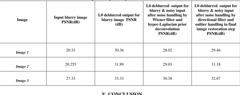
A comparison of estimated kernels with ground truth kernels for two of the test images is shown in Fig. 4. It can be seen that the estimated kernel is indeed very much closer to the ground truth for our method. Table 1 shows the PSNR values of the experimental results obtained for blurry images as well as blurry & noisy images with noise handling. The proposed method is seen to produce good visual quality results with high improvement of PSNR values and no ringing artifacts even in the presence of noise. Most of the existing methods fail to produce such high PSNR values without the use of explicit edge prediction steps like shock filter, in the presence of noise.
(a)Estimated kernels (b)Ground truths
Fig 4: Comparison of estimated kernels with ground truth
Table 1: PSNR values of experimental results of our method for blurry images as well as for blurry & noisy images. The results of our method using directional filtering and outlier handlingare compared to the results using Wiener
filtering and Laplacian prior deconvolution.
Image Input blurry image
PSNR(dB)
L0 deblurred output for blurry image PSNR
(dB)
L0 deblurred output for blurry & noisy input after noise handling by
Wiener filter and hyper-Laplacian prior
deconvolution PSNR(dB)
L0 deblurred output for blurry & noisy input after noise handling by
directional filter and oultier handling in final
image restoration step PSNR(dB)
Image 1 20.33 30.36 28.02 29.46
Image 2 20.255 31.89 29.03 31.18
Image 3 27.33 33.33 30.38 32.67
V. CONCLUSION
In this paper, we propose a new single image deblurring technique that is robust to noise and produces good quality latent images with no ringing artifacts in the presence of noise. Our method uses directional filtering for noise handling which does not affect the blur information and the kernel estimation process significantly in an adverse manner. A loss function approximating L0 cost is used as a prior for regularization in the objective function, which produces an
deconvolution step with outlier handling is incorporated in the latent image restoration, in order to obtain a better quality image which is devoid of ringing artifacts and has much finer details. The method is very effective in handling blurry & noisy images compared to the existing deblurring techniques which deteriorates in performance when noise is present. As a future scope, the method can be extended to handle non-uniform blur in the presence of noise.
REFERENCES
[1] A. Levin, Y. Weiss, F. Durand and W. T. Freeman, "Understanding and evaluating blind deconvolution algorithms," International Conference on Computer Vision and Pattern Recognition (CVPR), pp.1964-1971,2009.
[2] J. H. Money and S. H. Kang, "Total variation minimizing blind deconvolution with shock filter reference," Image and Vision Computing, vol. 26, no. 2, pp. 302–314, 2008.
[3] S. Cho and S. Lee, "Fast motion deblurring," ACM Transactions on Graphics (SIGGRAPH ASIA), vol. 28, no. 5, p. article no. 145, Dec. 2009. [4] L. Xu and J. Jia," Two-phase kernel estimation for robust motion deblurring,” European Conference on Computer Vision (ECCV), pp. 157–
170,2010.
[5] L. Xu, Q. Yan, Y. Xia and J. Jia, "Structure extraction from texture via relative total variation," ACM Transactions on Graphics (SIGGRAPH ASIA), vol. 31, no. 6, 2012.
[6] J. Jia, "Single image motion deblurring using transparency," International Conference on Computer Vision and Pattern Recognition (CVPR), pp. 1-8,2007.
[7] N. Joshi, R. Szeliski and D. J. Kriegman, "PSF estimation using sharp edge prediction," International Conference on Computer Vision and Pattern Recognition (CVPR), pp. 1-8, 2008.
[8] M. Hirsch, C. J. Schuler, S. Harmeling and B. Scholkopf, "Fast removal of non-uniform camera shake," International Conference on Computer Vision ( ICCV), pp. 463–470, 2011.
[9] D. Krishnan, T. Tay and R. Fergus, "Blind deconvolution using a normalized sparsity measure," International Conference on Computer Vision and Pattern Recognition (CVPR), pp. 233–240,2011.
[10] L. Xu, S. Zheng and J. Jia, "Unnatural l0 sparse representation for natural image deblurring," International Conference on Computer Vision and Pattern Recognition (CVPR), pp. 1107–1114,2013.
[11] D. Kundur and D. Hatzinakos, "Blind image deconvolution", IEEE Signal Processing Magazine, 1996.
[12] R. Fergus, B. Singh, A. Hertzmann, S. T. Roweis and W. T. Freeman," Removing camera shake from a single photograph," ACM Transaction on Graphics (SIGGRAPH ASIA), vol. 28, no.5, pp. 787–794, 2006.
[13] Q. Shan, J. Jia, and A. Agarwala, "High-quality motion deblurring from a single image,"ACM Transactions on Graphics (SIGGRAPH ASIA),vol. 27,no. 3,2008.
[14] J. Pan, Z. Hu, Z. Su, M. H. Yang, "Deblurring Text Images via L0-Regularized Intensity and Gradient Prior," International Conference on Computer Vision and Pattern Recognition (CVPR), pp. 2901-2908, 2014.
[15] L. Zhang, A. Deshpande and X. Chen, "Denoising vs. deblurring: Hdr imaging techniques using moving cameras," International Conference on Computer Vision and Pattern Recognition (CVPR), pp. 522-529, 2010.
[16] R. Koehler, M. Hirsch, S. Harmeling, B. Mohler and B. Scholkopf, "Recording and playback of camera shake: benchmarking blind deconvolution with a real-world database," European Conference on Computer Vision (ECCV), pp. 27–40,2012.
[17] A. Levin, Y. Weiss, F. Durand, and W. T. Freeman,"Efficient marginal likelihood optimization in blind deconvolution," International Conference on Computer Vision and Pattern Recognition (CVPR) ,pp. 2657–2664,2011.
[18] A. Buades, B. coll and J. Morel," A non-local algorithm for image denoising," International Conference on Computer Vision and Pattern Recognition (CVPR), pp. 60-65,2005.
[19] L. Zhong, S. Cho, D. Metaxas, S. Paris, and J. Wang, "Handling noise in single image deblurring using directional filters," International Conference on Computer Vision and Pattern Recognition (CVPR), pp. 612–619,2013.
[20] L. I. Rudin, S. Osher, and E. Fatemi, "Nonlinear total variation based noise removal algorithms," Physica. D, pp.259–268,Nov. 1992.
[21] A. Levin, R. Fergus, F. Durand, and W. T. Freeman, "Image and depth from a conventional camera with a coded aperture," ACM Trans. Graphics, vol. 26, no. 3, 2007.
[22] S. Harmeling, S. Sra, M. Hirsch, and B. Scholkopf, "Multi frame blind deconvolution, super-resolution, and saturation correction via incremental EM," In Proc. ICIP, pp. 3313–3316, 2010.
[23] L. Yuan, J. Sun, L. Quan, and H.-Y. Shum, "Progressive interscale and intra-scale non-blind image deconvolution,"ACM Trans. Graphics, vol. 27, no. 3, 2008.
[24] S. Cho, J. Wang, S. Lee, "Handling Outliers in Non-blind Image Deconvolution," International Conference on Computer Vision, pp. 1-8,2010. [25] A. Buades, C. B. and J.-M. Morel, "The stair casing effect in neighborhood filters and its solution," IEEE Transaction on Image Processing,
vol.15, pp. 1499-1505, 2006.
[26] L. Xu, C. Lu, Y. Xu and J. Jia, "Image smoothing via l0 gradient minimization,"ACM Transactions on Graphics (SIGGRAPH ASIA), vol. 30,