Vol. 2, Issue 10, October2013

(1)

Copyright to IJIRSET www.ijirset.com 5305

NUMERICAL SOLUTION FOR BOUNDARY

VALUE PROBLEM

USING FINITE DIFFERENCE METHOD

R.LAKSHMI1, M.MUTHUSELVI2

Assistant Professor, Department of Mathematics, PSGR Krishnammal College for women, Coimbatore ,Tamil Nadu, India1 Assistant Professor, Department of Mathematics, Dr.SNS Rajalakshmi College of Arts and Science, Coimbatore, Tamil Nadu,

India2

Abstract: In this paper, Numerical Methods for solving ordinary differential equations, beginning with basic techniques of finite difference methods for linear boundary value problem is investigated. Numerical solution is found for the boundary value problem using finite difference method and the results are compared with analytical solution. MATLAB coding is developed for the finite difference method. The results are reported for conclusion.

KEYWORDS: Ordinary Differential Equations, finite Difference method, Boundary value problem, Analytical solution, Numerical solution

I. INTRODUCTION

In mathematics, finite-difference methods are numerical methods for approximating the solutions to differential equations using finite difference equations to approximate derivatives. Finite differences method is used in soil physics problems. An important application of finite differences is in numerical analysis, especially in numerical differential equations, which aim at the numerical solution of ordinary and partial differential equations respectively. The idea is to replace the derivatives appearing in the differential equation by finite differences that approximate them. The resulting methods are called finite difference methods. Common applications of the finite difference method are in computational science and engineering disciplines, such as thermal engineering, fluid mechanics, etc.

A. STEPS INVOLVED IN FINITE DIFFERENCE METHOD

A finite difference method typically involves the following steps: Generate a grid, for example ( ; t (k)), where we want to find an approximate solution.

 Substitute the derivatives in a system of ordinary differential equations with finite difference schemes.  The ordinary differential equation then becomes a linear/non-linear system of algebraic equations.  Solve the system of algebraic equations. Implement and debug the computer code.

 Do the error analysis, both analytically and numerically.

B. DERIVATION OF FINITE DIFFERENCE METHOD

Let consider the linear equations

x





p t x t

( ) ( )





q t x t

( ) ( )



r t

( )

(1) With boundary condition x (a) = α and x (b) = β.

To start the derivation first replace each term x (tj) = xj

(2)

And the formula for central difference formula for first derivative

Gives, substitute x (tj) = xj in the above equation, and get 1 1 2

( )

2

j j

j

x x

x o h

h

  

  

(3)

Now consider the second derivative of central difference formula equation

1 1 2

2

( ) 2 ( ) ( )

( )j j j j ( )

x t x t x t

x t o h

h

   

  

(4)

Substitute x (tj) = xj in equation (4) and get

1 1 2

2

( )

j j j

j

x x x

x o h

h

   

  

(5)

Substitute equation (3) and (5) in (2) get,

1 1 2 1 1 2

2 2

( ) ( )( ( )) ( ) ( ) 2

j j j j j

j j j j

x x x x x

o h p t o h q t x r t

h h

    _ _    _ _ _

(6)

Next, drop the two terms in o (h2) in equation (6)

1 1 2 1 1

2

2 ( )

( )(

)

( )

2

j j j j j

j j j j

x

o h

p t

q t x

r t

h









_

_





_

(7)

And introduce the notation pj = p(tj), qj= q(tj) and rj = r(tj) in equation (7). This produces the difference equation

1 1 1 1

2

( )

2

j j j j j

j j j j

x x x x x

p q x r

h h

    _    _ _ ₍₈₎

this is used to compute numerical approximation to the differential equation. This is carried out by multiplying each side of (8) by h2, and then collecting terms involving xj-1, xj and xj+1 and arraying them in a system of linear equations.

(7) multiply by h2 gives

1 1 2 2 1 1

2

2 (

)

[

(

)

]

2

j j j j j

j j j j

x

h

p

q x

r

h









_





_

2 2

1

2

1 1 1

2

j j j j j j j j j j

h

x

_



x



x

_



p x

_



p x

_



h q x



h r

(9)

equation (9) multiply by -1

2 2

1 2 1 1 1

2 2

j j j j j j j j j j

h h

x_ x x_ p x_ p x _ h q x h r

       

Now collecting the term xj-1, xj and xj+1

2 2

1 1

( 1) (2 ) ( 1)

2 j j j j 2 j j j

h h

p x_ h q x p x_ h r

        (10)

for j = 1,2,…N-1 in equation (10). when j = 1

2 2

1 0 1 1 1 2 1

( 1) (2 ) ( 1)

2 2

h h

p x h q x p x h r

        (11)

And x0 = α the equation (11) becomes

2 2

1 1 1 1 2 1

( 1) (2 ) ( 1)

2 2

h h

p  h q x p x h r

       

2 2

1 1 1 2 1 1

(2 ) ( 1) ( 1)

2 2

h h

h q x p x h r p 

      

2 2

1 1 1 2 1

(2 ) ( 1)

2 o

h

h q x p x h r e

     

(3)

Copyright to IJIRSET www.ijirset.com 5307 where 0 1 ( 1) 2 h

e  p 



when j = N-1

2 2

1 2 1 1 1 1

( 1) (2 ) ( 1)

2 N N N N 2 N N N

h h

p _ x _ h q _ x _ p _ x h r _

       

And xN = β, then the equation (13) becomes

2 2

1 2 1 1 1 1

2 2

1 2 1 1 1 1

( 1) (2 ) [ 1]

2 2

( 1) (2 ) [1 ]

2 2

N N N N N N

h h

p x h q x h r p

h h

p x h q x h r p

                             

 

h r

2 _N_₁



e

_N

2 2

1 2 1 1 1

( 1) (2 )

2 N N N N N N

h

p _ x _ h q _ x _ h r _ e

       (13) where 1 [1 ] 2 N N h

e   p _



The system in equation (10), (12), (13) shows how the familiar triangle is formed, which is more visible when displayed with matrix notations

2 1 1

2

2 2 2

2

3 3 3

2

2 2 2

2

1 1

2 1 0 0 ... 0 ... 0

2

1 2 1 0 ... 0 ... 0

2 2

0 1 2 1 ... 0 ... 0

2 2

0 0 1 2 1 ... 0

2 2

0 0 0 1 2 1 0

2 2

0 0 0 0 ... ... 1 2

2

j J j

N N N

N N

h h q p

h h

p h q p

h h

p h q p

h h

p h q p

h h

p h q p

h

p h q

                          2 1 0 1 2 2 2 2 3 3 2 2 2 ₂ 2 1 ₁ j j N _N N N N

h r e

x

h r x

x h r

x _{h r}

x _{h r} _e

 _  _      _ _   __ _   _ _   _ _   _ _   _ _  _      _ _   _ _   __ _   _ _  

    ₍₁₄₎

where ₀

(

₁

1)

2 h

e



p





and

(

₁

1)

2

N N

h

e





p

_





II. FINITE DIFFERENCE METHOD FOR SOLVING BOUNDARY VALUE PROBLEM

2 2

2

2 ( )

( )

1

1 t

x

t

x t

t





_





_



with x(0) = 1.25 and x(4) = -0.95 over the interval [0,4].

A. NUMERICAL SOLUTION FOR BOUNDARY VALUE PROBLEM

The given equation is

2 2

2

2 ( )

( )

1

1 t

x

t

x t

t











(15)

And consider the linear equation

(4)

comparing equations (15) and (16) the values of pj , qj , rj are obtained. Approximation solution for boundary value problem using finite difference method.

2 2

1 1

( 1) (2 ) ( 1)

2 j j j j 2 j j j

h h

p x_ h q x p x_ h r

       

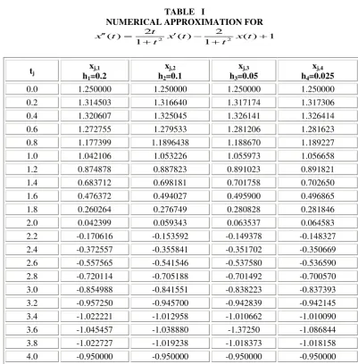
The finite-difference method is used to construct numerical solutions {x j} using the system of equations (10).There are 41 terms in the sequence generated with h_{2 = 0.1, and the sequence {x}_{j, 2}} only includes every other term from these computations; they correspond to the 21 values of {t j} given in Table 1. Similarly, the sequences {x _j.3} and {xj, 4 } are a portion of the values generated with step sizes h3= 0.05 and h_{4 = 0.025, respectively, and they correspond to the 21 values} of {t j } in Table 1.

B. ANALYTIC (OR) EXACT SOLUTION FOR THE BOUNDARY VALUE PROBLEM

Next compare numerical solutions in Table 1 with the analytic solution. Let consider the equation (15), integrating twice with respect to t to the limit 0 to 4 .

x(t)= 1.25+0.486089652t −2.25t2+2tarctan(t)− ln (1+t2) +t 2ln (1+t) (17) Put t=0 ,x(0)=1.25000. Continuing this process the values are presented in the below table. Comparing the values of x (t), in

Table 1 and Table 2. The numerical solutions have error of order o (h2).

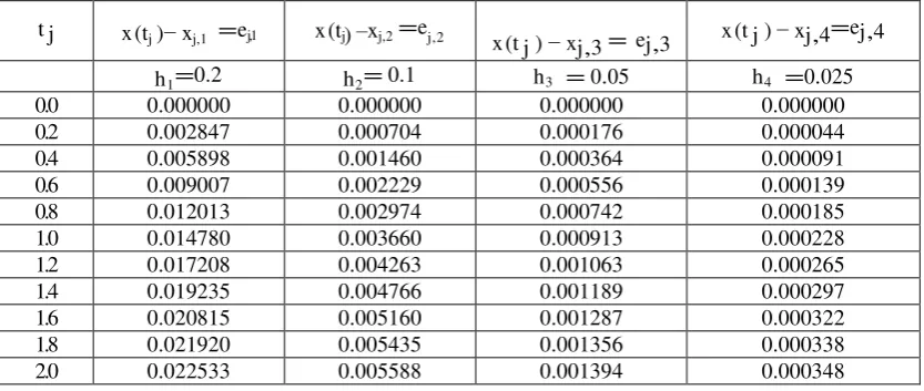
C. ERRORS IN NUMERICAL APPROXIMATION USING FINITE DIFFERENCE METHOD

Hence reducing the step size by a factor of results in the error being reduced by about . For instance, at tj = 1.0 the errors incurred with step sizes h1=0.2, h2 =0.1, h3 =0.05, and h4 =0.025 are

ej.1 = x(tj) – xj,1 = 1.056886 - 1.042106 = 0.014780, e j.1 = 0.014780 e j,2 = x(tj) exact – xj,2 = 1.056886 - 1.053226 =0.003660, e j,2 = 0.003660 e j,3 = x(tj) – xj,3 = 1.056886 - 1.055973 = 0.000913, e j,3 = 0.000913 and e j,4 = x(tj) – xj,4 = 1.056886 - 1.056658 = 0.000228, e j,4 = 0.000228 Their successive ratios

and .

are approaching . A careful scrutiny of Table 3 will reveal that this is happening. And FIGURE-I shows that the difference between the numerical approximation solution and analytic solution.

D. RICHARDSON’S IMPROVEMENT SCHEME

Richardson’s improvement scheme can be used to extrapolate the seemingly inaccurate sequences {xj,1}, {x j,2}, {xj,3}, and {xj,4} and obtain six digits of precision. Eliminate the error terms o(h2) and o((h/2)2) in the approximations {x j,1} and {xj,2} by generating the extrapolated sequence

{zj,1} = {(4xj,2 – xj,1) / 3}. (18) Similarly, the error terms o((h/2)2) and o((h/4)2) for {xj,2} and {xj,3} are eliminated by generating

{zj,2} = {(4xj,3 – xj,2) / 3} (19) It has been shown that the second level of Richardson’s improvement scheme applies to the sequences {zj,1} and {zj,2} so the third improvement is

= {(16z j,2 − z j,1) / 15} (20) Now illustrate the situation by finding the extrapolated values that correspond to = 1.0. The first extrapolated value is

(5)

(22)

Finally, the third extrapolation involves the terms zj,1 and z j,2 :

(23)

This last computation contains six decimal places of accuracy. The values at the other points are given in Table 4.

E. MATLAB PROGRAM FOR FINITE DIFFERENCE METHOD USING SCRIPT FILE

clc;

% problem definition aa=0;

bb=4; n=20;

alpha=1.25;beta=-0.95; h=(bb-aa)/n;

t=zeros(1,n+1); x=zeros(1,n-1); a=zeros(1,n-2); b=zeros(1,n-1); c=zeros(1,n-2); d=zeros(1,n-1); t=aa+h:h:aa+h*(n-1);

p=(2*t/(1+t.^2)).*ones(1,n-1); q=(-2/(1+t.^2)).*ones(1,n-1); r=1*ones(1,n-1);

% end problem definition x=linspace(aa+h,bb,n); a=zeros(1,n-1);

a(1:n-2)=-1-p(1,1:n-2)*h2; d=(2+hh*q);

b=zeros(1,n-1);

b(2:n-1)=-1+p(1,2:n-1)*h2; c(1)=hh*r(1)+(1+p(1)*h2)*alpha; c(2:n-2)=-hh*r(2:n-2);

c(n-1)=hh*r(n-1)+(1-p(n-1)*h2)*beta; x=trimat(a,d,b,c);

tt=[aa t bb]; xx=[alpha x beta]; out=[tt' xx']; disp(out)plot(tt,xx) grid on

F. MATLAB program for solving Tridiagonal systems using function file program

function x=trimat(A,D,C,B)

(6)

% - C is the super diagonal of the co-efficient matrix % - B is the constant vector of the linear system %Output- x is the solution vector

N=length(B); for k=2:N

mult=A(k-1)/D(k-1) D(k)=D(k)-mult*C(k-1); B(k)=B(k)-mult*B(k-1); end

x(N)=B(N)/D(N); for k=N-1:-1:1

x(k)=(B(k)-C(k)*x(k+1))/D(k); end

TABLE I

NUMERICAL APPROXIMATION FOR

2 2

( ) ( ) ( ) 1

1 1

t

x t x t x t

t t

  _   _ 

tj

xj,1 h1=0.2

xj,2 h2=0.1

xj,3 h3=0.05

xj,4 h4=0.025

0.0 1.250000 1.250000 1.250000 1.250000

0.2 1.314503 1.316640 1.317174 1.317306

0.4 1.320607 1.325045 1.326141 1.326414

0.6 1.272755 1.279533 1.281206 1.281623

0.8 1.177399 1.1896438 1.188670 1.189227

1.0 1.042106 1.053226 1.055973 1.056658

1.2 0.874878 0.887823 0.891023 0.891821

1.4 0.683712 0.698181 0.701758 0.702650

1.6 0.476372 0.494027 0.495900 0.496865

1.8 0.260264 0.276749 0.280828 0.281846

2.0 0.042399 0.059343 0.063537 0.064583

(7)

TABLE II

EXACT SOLUTION FOR THE GIVEN BOUNDARY VALUE PROBLEM

tj x (tj)

0.0 1.2500

0.2 1.317350 0.4 1.326505

0.6 1.28762

0.8 1.189412 1.0 1.056886 1.2 0.892086 1.4 0.702947 1.6 0.497187 1.8 0.282184 2.0 0.064931 2.2 -0.147977 2.4 -0.350325 2.6 -0.536261 2.8 -0.700262 3.0 -0.837116 3.2 -0.941888 3.4 -1.009899 3.6 -1.036709 3.8 -1.018086 4.0 -0.950000

TABLE III

ERRORS IN NUMERICAL APPROXIMATIONS USING THE FINITE-DIFFERENCE METHOD

t j x (tj₎− xj,1 =e_j,1 x (tj₎–xj,2 =ej,2

x (t j ) − xj,3 = ej,3 x (t j ) − xj,4=ej,4 h1=0.2 h2= 0.1 h3_{= 0.05} h4_=0.025

0.0 0.000000 0.000000 0.000000 0.000000

0.2 0.002847 0.000704 0.000176 0.000044

0.4 0.005898 0.001460 0.000364 0.000091

0.6 0.009007 0.002229 0.000556 0.000139

0.8 0.012013 0.002974 0.000742 0.000185

1.0 0.014780 0.003660 0.000913 0.000228

1.2 0.017208 0.004263 0.001063 0.000265

1.4 0.019235 0.004766 0.001189 0.000297

1.6 0.020815 0.005160 0.001287 0.000322

1.8 0.021920 0.005435 0.001356 0.000338

(8)

2.2 0.022639 0.005615 0.001401 0.000350

2.4 0.022232 0.005516 0.001377 0.000344

2.6 0.021304 0.005285 0.001319 0.000329

2.8 0.019852 0.004926 0.001230 0.000308

3.0 0.017872 0.004435 0.001107 0.000277

3.2 0.015362 0.003812 0.000951 0.000237

3.4 0.012322 0.003059 0.000763 0.000191

3.6 0.008749 0.002171 0.000541 0.000135

3.8 0.004641 0.001152 0.000287 0.000072

4.0 0.000000 0.000000 0.000000 0.000000

TABLE IV

EXTRAPOLATION OF THE NUMERICAL APPLICATIONS {XJ,1 }, {XJ,2 },{XJ,3 } OBTAINED WITH THE FINITE DIFFERENCE METHOD.

tj

x (t j₎ Exact solution

(9)

0 0.5 1 1.5 2 2.5 3 3.5 4

-1.5 -1 -0.5 0 0.5 1 1.5

t

x(

t)

Numerical approximation solution Exact solution

Fig. I Comparing the solution of numerical approximation solution, exact solution and solution of the finite difference method using MATLAB program to the given boundary value problem

III. CONCLUSION

A boundary value problem is solved using finite difference method and is verified with exact solution. It is found that the results are agreed with exact solution.

REFERENCES

[1].John H.Mathews , Kurtis D. Fink, Numerical Methods Using MATLAB, Fourth Edition,2008, Published by Dorling Kindersley(INDIA)Pvt.Ltd., New Delhi.

[2].DR. M. K. Venkataraman, Numerical Methods in Science And Engineering, Fifth Edition (Revised & Enlarged ), 2004, The National Publishing co., Chennai.