Article
1
Chaotic Synchronizing Systems with Zero Time
2
Delay and Free Couple via Iterative Learning Control
3
Chun-Kai Cheng and Paul C.-P. Chao *
4
Institute of Electrical and Control Engineering, National Chaio Tung University, Taiwan;
5
[email protected] (C. K. Cheng)
6
* Correspondence: [email protected]; Tel.: +886-3-513-1377
7
Abstract: This research not only dedicated a less restrictive method of iteration-varying function for
8
a learning control law to design a controller but also synchronize two nonlinear systems with free
9
time-delay. In addition, the mathematical theory of system synchronization has proved rigorously
10
and the theory verified through an example to demonstrate the behavior of each parameter in the
11
theory. The design of a controller using the iterative learning control law is significant for robotic
12
tracking. The controller in this research generates a feed-forward control input using the error
13
dynamics among the drive-response systems. The error dynamics satisfies the Lyapunov function
14
and the combination of output errors, which respectively represented relative estimated differences
15
of the drive-response systems. The iterative learning control rule serves the function of a filter
16
adding previous control error after the end of each iteration. The numerical example of a
17
synchronous system is given a Lorenz system for driving and another with the iterative learning
18
control law for response under different initial condition. The results verify and demonstrate the
19
proposed mathematical theory. The simulation exhibits consistency in the behavior of each
20
parameter to match mathematical theory.
21
Keywords: synchronization; chaos; chaotic system; Iterative Learning Control (ILC); Lyapunov
22
function; error convergent
23
24
1. Introduction
25
The concept of Iterative Learning Control (ILC) theory [1] takes the errors of a system repeatedly
26
executing similar tasks into consideration to improve overall performance by learning previous
27
information of the original system. The system's learning control regards the same multiple
28
operations under various operating conditions [1-2]. To conduct a betterment process for a
29
mechanical robot is the original principle of ILC in 1984 [3]. The ILC differs from other learning
30
control systems, such as repetitive control, adaptive control, and neural network [2] that it will adjust
31
the input signal according to previous output of the same system whereas to modify the controller is
32
an example of an adaptive control stages [2-3]. Instead, many studies described the iterative control
33
process by mphasizing its periodic control and not considering its "Learning" process [2].
34
ILC is applicable to many fields in system modeling, PID-control, nonlinear dynamical system,
35
and system synchronization as well as in the academic field [4-8]. Maria [9] also proposed the iterative
36
method by using many theories of classical linear system to approximate nonlinear systems. Recently,
37
the ILC theory has also employed chaotic secure communication into encrypt and decrypt a message
38
[4]. ILC also becomes the focus of many industrial systems for manufacturing, robotics, and assembly
39
line entailing repetition of mass production [1-2].
40
The goal of designing ILC controller is to generate a feed-forward control signal as an
41
appropriate tracking reference to proceed or deny a repeating distance, which can improve the
42
performance of systems and achieve low tracking error, while the tracking error exists on every
43
transient-time repeated work [1]. Arimoto in the [3] examined the PID-type learning algorithm of
44
betterment process during the operation of robots and ensured the error of system was convergent.
45
Kuc [5] proposed the learning rule of nonlinear dynamic systems was through each iteration of linear
46
feedback by uniformly bounded state error to track reference input. The iterative method of classical
47
linear system theory was introduced by Mara [10] to approximate the nonlinear systems.
48
The betterment effect of iterative process [3] shows convergence in the vector-norm of errors,
49
but the iterative learning control is not unique to non-linear system. The Lyapunov function provides
50
the sufficient condition for convergence [2-3]. The tracking error is the asymptotically stable system
51
is a bounded function constructed by Lyapunov function [1]. The Lyapunov function is the most
52
commonly used strategies to study the stability of a control system. The Lyapunov function in [11]
53
serves to guarantee the designed salve system in asymptotical synchronization with the master
54
system.
55
In this research, the principle of learning operator is in Hauser [12], and the Lyapunov function
56
of synchronization system follows the method by Zhou [13] for stability. The restrictive
57
synchronization criteria of the Lyapunov function exhibited in [14]. The existence and stability
58
conditions of two different continuous chaotic systems found in [16] and the synchronization
59
manifold of two unidirectional systems showed equivalent state vectors indicating the possible
60
perfect system synchronization [17]. The error norm in the dynamics error system would be
61
monotonically convergent when the Markov parameters were used to find the time-varying learning
62
gain [20], that such error convergence in dynamics systems was monotonic and independent of the
63
iteration time duration as shown in [21]. Therefore, the system with couple and time-delay to
64
synchronize was verified the stability by the Lyapunov function [13 -21].
65
This research dedicated a less restrictive method of iterative control learning law for the design
66
of controller to synchronize two distinct nonlinear systems, which are free time-delay and non-couple.
67
The rigorously proof of each parameter is in relative mathematical theory, such as the iterative
68
learning control law is bounded and non-increasing, the dynamics error system is stable, and the
69
tracking error between the drive and response systems is convergent. The results of example
70
indicated the behavior of parameters in the synchronous process. The numerical example for
71
synchronization of drive-response systems in which the drive is the Lorenz system [23] and response
72
is the similar system with the iterative learning law, respectively. Their initial conditions are different.
73
The results of example verify the theory in this paper and demonstrate the effectiveness of proposed
74
concept.
75
The relevant studies herein include the followings: (1) the description of synchronization system;
76
(2) the mathematically proof of related theory and proposed the scheme of iterative learning control;
77
and (3) the simulation results of example as verification of the proposed mathematical theory in
78
exhibiting the performance of ILC algorithm for system synchronization. Finally, this paper derives
79
a conclusion and recommendation for future works.
80
2. The ILC Problem Formulation
81
2.1. System Description
82
The drive and response systems are chaotic systems to synchronize with zero time delay and
83
free couple and the general formula of systems are described by following equations equation (1a)
84
and equation (1b), respectively.
85
( ) = ( , ) = ( ) ( ),
( ) = ( ),
(1a)
The response system adjusts the error between the drive and tracking systems approaching
86
synchronization using the control input ( ).
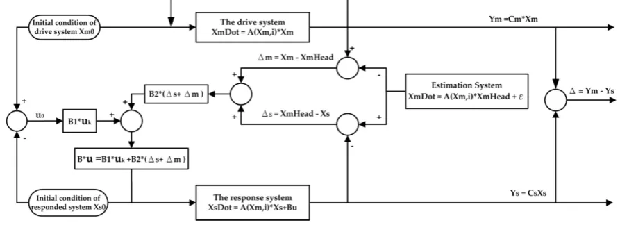
87
( )( ) = ( ), + ( )( ) = ( ) ( )( ) + ( )( ),
( )( ) = ( )( ),
The state vectors ( ), ( )( ) and the outputs and ( ) are of the drive-response systems
88
in state space , respectively. Originally, ( , )and ( ), are similar systems. The response
89
system with the iterative control input signal of ( )( ) and the output ( ), after the k-th learning
90
of iteration. The Cm , Cs, and B = BT are nonsingular constant matrices with appropriated dimensions
91
and some entries of the nonsingular polynomial matrix ( ) are replaced by the i-th component
92
of ( ) to be the factor of system synchronization, where i = 1, 2, 3. The input signal
93
sequence ( )( ) , ,… in is the control learning law after the k-th iterative learning for the
94
response system synchronizing the drive system.
95
( )= − ( ) is the synchronization error and the output error of drive-response system is
96
given − ( )= − ( ). The output error is equal to the synchronization error when
97
= = is set. The dynamical system synchronization error between drive-response systems can
98
be described in (1a) and (1b).
99
( )= ( ) − ( )( ) = ( ) − ( ) + ( )( ) = ( ) ( )+ ( )( ),
(2)
The the appropriate ( )( ) is given and the minus in (2) is absorted by B. The limitation of
100
synchronization error must approach to zero that islim n→∞
( )= ( )− = 0, and the error dynamics
101
should be less than or equal to zero, that is Δ ≦ 0 , when iteration learning procedure applies to
102
response system to track drive system in the time interval [0, T] after sufficiently large iterative
103
number k.
104
The characters between drive and response systems are the drive system to be reference system
105
and the tracking system for a response system in synchronization procedure, respectively. The
106
response system traces the trajectory of the drive system by employing the output information of
107
drive system. In order to achieve the goal of synchronization and search a system whose trajectory is
108
closed to drive system, it is necessary to find an estimated system similar to drive system. The
109
estimated system in [21] can be defined the measuring system of drive system as (3).
110
( ) = ( , ) + = ( ) ( ) + , (3)
The nonlinear problem is no general solution. The perturbation and linearization techniques will
111
be applied to the equation (3). Least square linear estimation is familiar to minimize the errors in
112
measure processes. The error criterion of equation (3) defined as
113
( ) = = ( ) − ( ) ( ) ( ) − ( ) ( ) , (4)
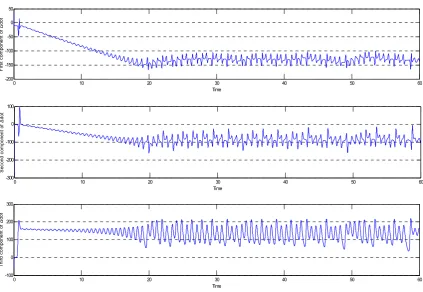
The minimization of E is to differentiate E with respect to the state vector and equate to the result
114
as:
115
= − ( ) ( ) + ( ) ( ) ( ) = ,
( ) = ( ) ( ) ( ) ,
(5)
The parameter ( ) is the minimum value of the scale of error E.
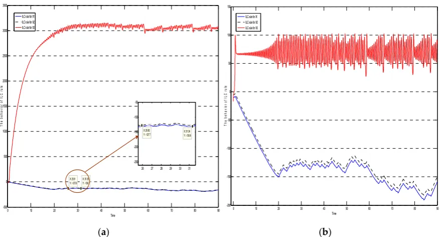
116
The design of the Lyapunov function reaches the synchronization of the chaotic system whose
117
manifold = ( )must be stable [13-17]. This fact indicates systems synchronization of (1a) and
118
(1b) through ILC procedure so that the error dynamics as (2) is stable by Lyapunov criterion and the
119
local Lipschitz condition is satisfied during the period of the system.
Lemma 1. The equation (2) has a trivial solution by the ILC procedure. ( , ) (1a) and
121
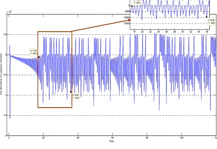
( ), in (1b) are satisfied local Lipschitz condition in the interval [0, T].
122
Proof:
123
By the ILC procedure, there is a trivial solution ( )= − ( ) = 0
which implies δ > 0 for all
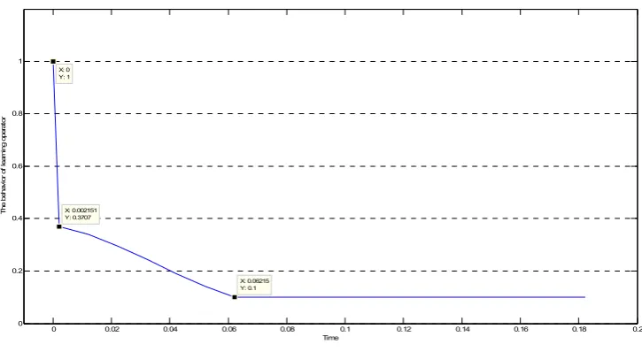
124
ε > 0 and k = 0, 1, 2,… such that ‖ ( , ) − ( ( ), )‖ < as ‖ − ( )‖ < which means the
125
condition ‖ ( , ) − ( ( ), )‖ < ‖ − ( )‖ is held. The ( , ) is convergent to
126
( ), when ( )= − ( ) approaches to zero. Basically, the consequence of this lemma implies
127
that ‖ ( , ) − ( ( ), )‖ < → 0.
128
□
129
The convergence of synchronization error, ( ),indicates the error dynamics ( ) is
non-130
increasing that is ( )≤ 0 and dependent on the iterative learning control law ( )( ) in (1a) is chosen
131
as
132
( )( ) = ( )( ) + ( + ( )) = ( )( ) + ( ),
(6)
where the and are appropriate constant matrices and symmetry. The learning law ( ) is
133
previous of ( ). = ( − ) and ( )= − ( ) are the errors between the estimated state
134
vectors and the state vectors of and ( ), respectively.
135
□
136
The sum of errors of equation (6) is + ( )= ( ). If the error dynamics in the equation (2) is
137
convergent then the iterative learning control law ( )( ) is decremented. The completed proof is
138
going to exhibit in lemma 2.
139
Lemma 2. If the error dynamics in the equation (2) is convergent then the iterative learning
140
control law in the equation (6) is non-increasing function.
141
Proof:
142
From equation (5) and lemma 1, the error in (2) can be rewrite as following
143
( )= ( − ) + − ( ) = + ( ),
(7)
Suppose that ( − ) ≤ and − ( ) ≤ , take the = , , the equation
144
(7) can be rewritten the detail as ( )= ( − ) + − ( ) = + ( )≤ . The
145
difference of iterative learning control law is ( )( ) − ( )( ) = ( )≤ ( ) ≤ ‖ ‖ ( ) =
146
0 which means the sequence ( )( ) , ,,⋯ is non-increasing because the error ( ) is convergent
147
to zero.
148
□
149
The analytical approximation of the chaotic systems synchronizing the trajectory in equations
150
(1a) and (1b) is the Lyapunov stable investigating [13-17]. The Lyapunov criterion introduced in the
151
theorem 1 is a positive-definite function with non-time delay and free couple of the system (2).
152
Theorem 1. The iterative learning control law is chosen as the equation (6). The Lyapunov
153
function can be defined as
154
( )( ) = ( ) ( ) + ( ) ( ) ,
(8)
(a). When = , ( )( ) = ( ) ( ) is the Lyapunov function of an estimation system in the
155
system (3).
156
(b). If ( )( ) is Lyapunov function of the system (2) then the system should be stable.
157
Proof:
First part of proof is to prove the part (a) in this theorem. The derivative of the function ( )( )
159
along the track of the system (2) was in [24] discussion and written as
160
( )( ) = ( ) ( ) ,
(9)
By using the lemma 1, the equation (9) has a trivial solution. The derivative of Lyapunov function is
161
equal to zero or negative, which implies that the system (2) is stable.
162
Next, the proof of part (b) is a general case of a chaotic system with no time-delay and free couple.
163
The derivative of the function ( )( ) along the track of the system (2) is introduced in [13 -17] and
164
following as:
165
( )( ) = ( ) ( ) + ( )( ) ( )( ) − ( )( ) ( )( )
= ( ) ( ) + ( )( ) − ( )( ) . (10)
The first term in equation (10) proved in the equation (8) and the second term should be equal
166
to zero or negative when the iterative learning control law is a non-increasing function. When the
167
iterative control learning is divergent, the Lyapunov function of the dynamical system (1a) and (1b)
168
would be divergent and the system (2) cannot be stable.
169
□
170
In the proof of the theorem, it is important to determine the learning control law, u(k)(t), in
171
Lyapunov function applied in the more complex system. The decision as to what suitable for iterative
172
learning control law and parameters B1 and B2 to reduce the divergence of non-linear systems should
173
be discussed and studied the synchronization of non-linear systems.
174
2.2. Proposed algorithm for Iterative Learning Control Law
175
The iterative learning control algorithm exhibits in figure 1. The diagram contains three systems,
176
namely the drive system, the response system, and the estimated system, with three outputs, namely
177
the output of drive system, the output of response system and the output of error, respectively. The
178
initial conditions of the drive system and the response system are different. The iterative learning
179
control law of the first stage exhibits the error of initial conditions between the drive system and the
180
response system. The estimation system in the equation (3) provides for the estimated state vectors
181
as expressed equation (4), to drive and response systems, respectively. The drive system and the
182
response system are in closed-loop that the feedback in the former is the own output of drive system
183
and the feedback in the latter is the result of iterative learning control law as the own output of
184
response system.
185
186
Figure 1. The iterative learning control algorithm
The algorithm in the figure 1 of examines learning control input u(k) is bounded convergence and
188
satisfies the criteria of monotonically convergent conditions. The learning control input u(k) in the
189
equation (6) is concerned with the ability to adjust the feedback error of response system and track
190
the trajectory of the drive system. Therefore, iterative learning control law, u(k), must be bounded.
191
Corollary 1. The learning control input u(k) in the equation (6) is monotonic decreasing and
192
bounded.
193
Proof:
194
The learning control law in equation (5) is a updated law to refresh the input of the system (1b)
195
proposed. The sequence ( )( ) , ,,⋯ is non-increasing sequence such that the condition
196
( )( )
= , ,,⋯=
(0)( ) ≤ is held with an upper bounded M of real number having in
197
lemma 2.
198
The appropriate matrices B, B1, and B2 making the sequence ( )( ) , ,,⋯ is strictly decreasing
199
are important. The ILC law ( )( ) , ,,⋯ can be expanded it in initial learning law ( )( ) by
200
induction as follows:
201
( )( ) = ( ) ( )( ) + ( ) ( )+ ( ) ( )+ ⋯ + ( ),
(11)
The learning operator L in this research follows the method of Hauser [12] as:
202
≡ ( ∗ ) (12)
‖ − ‖ ≤ < 1. (13)
The consequence is from the monotonically decreasing sequence ( )( ) , ,,⋯ of the ILC rule.
203
The u(0) is the maximum in the monotonically decreasing sequence ( )( )
, ,,⋯ and ‖ ‖ ≤ 1 in
204
equation (13) . Theses matrices can be found by Linear Matrix Inequality (LMI) method, but not main
205
object in this research.
206
□
207
3. Example Illustration and Demonstrated Results
208
The example in this section is going to demonstrate the results of synchronization approach,
209
investigate the non-linear drive-response systems with free time-delay and non-couple, and
210
synchronize two non-linear systems. The drive system is expressed by a Lorenz system as follows
211
[23] and the response system is another with the ILC input.
212
3.1. The Example of Iterative Learning Algorithm to Decide Learning Law
213
In order to exhibit the synchronization of two non-linear systems and verify the algorithm of
214
iterative learning control law in Figure 1, the drive-response systems with non-identical initial
215
conditions are given by follows:
216
( ) = ( , ) = ( ) ( ),
=
−10 10 0
30 −1
0 − 8 3 ( ),
( ) = ( ), ( = 0) = (0.02, 0.01, 0.03),
(15)
and
217
=
−10 10 0
30 −1
0 − 8 3
( ) + ( )( ),
( )( ) = ( )
( ), ( )= (2, 1, 3),
From the drive-response system, the error dynamical system is expressed as
218
( )= ( ) − ( )
= ( ) ( )+ ( )( ),
=
−10 10 0
30 −1
0 − 8 3
( )+ (− ) ∗ ( )( ),
(17)
In this example, setting the = = , the output error is − ( )= ( )= − ( ) in R3. The
219
paramaters are explained as = ( , , ) , ( )= ( ), ( ), ( ) , ( )= ( )− ( ) . The
220
in polynomial matrix ( ) is the first component of the state vector in the drive system. The
221
state vector in estimation system is ( ) = ( ) ( ) ( ) and the iterative learning law with
222
the initial condition ( )( = 0) = ( )( = 0) = − ( ) . The ( )( ) in equation (6) and Lyapunov
223
equation in equation (8), respectively. The matrices B1 and B2 in the ILC rule of equation (6) are as:
224
= 0 11 0 00
0 0
and =
0.1 0 0
0 0.1 0
0 0 − 3 8 , (18)
The metrix B1 has an entry with the minimal eigenvalue λ of polynomial matrix ( ).
225
The matrix B in the equation (1b) is easy to choose the identity matrix. The results were conducted
226
the simulations with MATLAB to verify the performance of ILC rule. The drive system is used an
227
ode45 funtion in simulink and the response system is found using the the Euller method with the
228
estimated state vectors of equation (5). The relevant simulation results show in the next section.
229
3.2. Simulation Results and Discussion
230
The trajectories in two-dimensional x1, x3-space of the drive system in black dash line, the
231
response system by estimating in red, and the estimation of drive system in blue show in the figure
232
2, respectively. The initial condition of drive system differs from others. The trajectory of estimated
233
systems quickly approach to the drive system after their initial condition but the approximation is
234
not excellent, just as the iterative learning controlled law is not perfect.
235
According to the equation (2) and lemma 2, the error dynamics ( )should be less than or equal
236
to zeor and the demonstration in the figure 3. The two previous components in ( ) are always
237
negative satisfied the error convergence criterion. Nevertheless, the third component is vibration in
238
the bounded interval around between 100 and 200 as well as to verify the bounded error of each
239
iteration and design appropriate controller by ILC rule in equation (2) and lemma 2.
Figure 2. The trajectories in two-dimensional x1, x3-space of systems.
241
Figure 3. Thesimulation of each component of the error dynamics system ( )
242
The behaviors of ILC rule in the Figure 4 show two components are always decreasing and
X3-243
component is non-increasing. The simulation results of equation (6) verify the lemma 2 and corollary
244
1. The behaviors are not identical for different ILC rule showed in the figure 5. The Figure 5a is
245
chosen the B1 is identity matrix and B1 = [0.1, 0.1, 0.92] in Figure 5b, respectively. One of components
246
is rose sharply and then the vibrating in a bounded interval and others are smoothly decreased in the
247
-20 -15 -10 -5 0 5 10 15 20 25
-40 -30 -20 -10 0 10 20 30 40 50 60
X2 Component
X
3
C
om
pon
ent
9 9.5 10
10 11 12 13 14 15 16 17
X: 9.874 Y: 14.99
X: 10 Y: 15
0.018 0.02 0.0220.0240.0260.028 -0.08
-0.06 -0.04 -0.02 0 0.02 0.04 X: 0.02Y: 0.03
X: 0.01928 Y: -0.02829
X: 0.0191 Y: -0.03171
Estimation System of Drive System Response System by estimating Drive System
The initial state of drive system The initial state of estimation system The estimated state of response system
0 10 20 30 40 50 60
-200 -150 -100 -50 0 50
Time
F
irs
t
co
m
pon
en
t
of
Δ
do
t
0 10 20 30 40 50 60
-300 -200 -100 0 100
Time
S
ec
on
d
co
m
po
nen
t
of
Δ
do
t
0 10 20 30 40 50 60
-100 0 100 200 300
Time
T
hi
rd
co
m
pon
en
t
of
Δ
do
previous ILC rule. In latter ILC rule exhibits one of components is more vibration in a bounded
248
interval than previous and the other decreasing components are speed bumps.
249
Figure 4. The brhavior of the iterative learning control law.
250
(a) (b)
Figure 5. The different behaviors of ILC with the different matrix B1 is list as: (a) B1 is identity
251
matrix; (b) B1 = [0.1, 0.1, 0.92].
252
The behavior of the derivative of Lyapunov function demonstrates in Figure 6 and the how
253
many time step of derivation Lyapunov function is less than zero or negative in the table 1, but the
254
number is notrelative to the different parameters μ in equation (10). The obvious phenomenon is to
255
regard the ILC rule to find an appropriate linear combination in equation (6) and the negative
256
derivative of Lyapunov function in equation (10). Lyapunov function is positive and non-increasing
257
function by the conditions of lemma 2 and corollary and the demonstration in Figure 6 has approached
258
the consequences and proved theorem 1. The curve in the Figure 7 demonstrates the behavior of Learning
259
0 10 20 30 40 50 60 70 80 90
-200 -150 -100 -50 0 50 X: 0.8222 Y: 14.07 Time X: 0.8222 Y: -2.938 X: 0.8122 Y: -7.658 X: 53.62 Y: -113.1 X: 58.82 Y: 11.54 X: 79.19 Y: 2.435 X: 58.51 Y: 1.888 T he beha vi or of it era tiv e lear ni ng cont ro l l aw
ILC rule for X1 ILC rule for X2 ILC rule for X3
0 10 20 30 40 50 60 70 80 90
-500 0 500 1000 1500 2000 2500 3000 3500 X: 25.9 Y: -127.8 Time T he b eh av io r of IL C r ul e X: 31.35 Y: -130.7
26 27 28 29 30 31 -250 -200 -150 -100 -50 X: 25.92
Y: -127.7 X: 31.34Y: -130.8 ILC rule for X1
ILC rule for X2 ILC rule for X3
0 10 20 30 40 50 60 70 80 90
-200 -150 -100 -50 0 50 100 150 Time T he beha vi or o f IL C r ul e
operator of ILC rule by using the formula in equation (12) in which the operator decreases rapidly to stable and
260
verifies the equation (14) is held.
261
Figure 6. The behavior of the derivative of Lyapunov function.
262
Table 1. The number of negative Lyapunov function with different values of μ.
263
Value of μ Negative Positive Total
1 9623 2377 12000
3 9637 2377 12000
10 9637 2373 12000
100 9629 2371 12000
264
0 20 40 60 80 100 120
-2 -1.5 -1 -0.5 0 0.5
1x 10
4
Time
T
he
de
riv
at
iv
e
of
Ly
apuno
v
func
tion
X: 35.95 Y: -9152 X: 17.48
Y: -583.3
18 20 22 24 26 28 30 32 34 36
-15000 -10000 -5000 0
X: 17.48 Y: -583.3
Figure 7. The behavior of the ILC rule..
265
4. Conclusions
266
This research exhibited the design of iterative learning controller and the results of simulation
267
with example to prove the mathematical theory of the chaotic system synchronization via iterative
268
learning control law. The demonstrations verified the mathematical theory as possible to
269
approximate the synchronization between systems. The ILC method is a convenient method to trace
270
the trajectory of systems, but it is not perfect tracking for all situations. In addition, the iterative
271
learning control law should be conditionally dependent on the system and would not be unique to
272
the specific system. It is a significant challenge to find coefficient matrices, which are the combination
273
of previous ILC law and trajectory error in this research, respectively. The ILC method could be use
274
for the non-linear system with time-delay and couple to adjust the learning control law and the
275
process should also applies to adaptive control, sliding mode control, and fuzzy control. The primary
276
research is essential for the tracking systems, such as robotic systems, secure communication systems,
277
image identification systems, and many others, which are part of the future developments and
278
applications.
279
Author Contributions: “Chun-Kai Cheng conceived and designed the simulation; Chun-Kai Cheng performed
280
the simulation; Chun-Kai Cheng analyzed the data; Chun-Kai Cheng and Paul C.-P. Chao wrote the paper.”
281
Conflicts of Interest: The authors declare no conflict of interest.
282
References
283
1. Bristow, D.A.; Tharayil, M.; Alleyne, A. G. A Survey of Iterative Learning Control, IEEE Control Syst. 2006,
284
26, 96 – 114.
285
2. Moore, K. L. Iterative Learning Control for Deterministic System, Springer: New York, USA, 1992, pp. 9 - 45,
286
ISBN: 3-540-19707-9
287
3. Arimoto, S.; Kawamura, S.; Miyazaki, F. Bettering Operation of Robots by Learning, Journal of Robotic
288
Systems, 1984, 1, pp. 123 - 140.
289
4. Acho, L. A Chaotic Secure Communication System Design Based on Iterative Learning Control Theory,
290
Appl. Sci. 2016, 6, pp. 311- 317.
291
5. Kuc, T. Y.; Lee, J. S.; Nam, K. An Iterative Learning Control for a Class of Nonlinear Dynamic Systems,
292
Automatica, 1992, 28, pp. 1215 - 1221.
293
6. Madady, A. An Extended PID Type Iterative Learning Control, Int. J. Control Autom. Syst. 2013, 11, pp.470
294
0 0.02 0.04 0.06 0.08 0.1 0.12 0.14 0.16 0.18 0.2
0 0.2 0.4 0.6 0.8 1
X: 0.002151 Y: 0.3707
Time
T
he
be
hav
ior
o
f
le
ar
ni
ng
o
per
at
or
X: 0.06215 Y: 0.1 X: 0
– 481.
295
7. Helfrich, B. E.; Lee, C.; Bristow, D. A.; Salapaka, S. M.; Ferreira, Placid M. Combined H-infinity-Feedback
296
control and Iterative Learning Control Design with Application to Nanopositioning Systems, IEEE
297
Transactions on Control Systems Technology, 2010, 18, pp. 336 - 351.
298
8. Liu, Z.; Wang, J.; Deng, B.; Wei, X.; Yu, H. Synchronization of Ghostburster neuron via Iterative Learning
299
Contol, 2014 7th IEEE International Conference on Biomedical Engineering and Informatics (BMEI), Bayshore
300
Hotel Dalian, China, 14-16 Oct. 2014.
301
9. María, T. R.; Banks, S. P. Linear, Time-varying Approximations to Nonlinear Dynamical Systems, Springer:
302
Berlin Germany, 2010, pp. 11 - 28.
303
10. Xu, J.X.; Yan, R.; Chen, Y.Q. On initial Conditions in Iterative Learning Control, IEEE Trans. Autom. Control,
304
2005, 50, pp. 1349–1354.
305
11. Cheng, C. K.; Kuo, H. H.; Hou, Y. Y.; Hwang, C. C.; Liao, T. L. Robust chaos synchronization of
noise-306
perturbed chaotic systems with multiple time delay, Physica A, 2008, 387, pp. 3093 - 3102.
307
12. Hauser, J. E. Learning control for a class of nonlinear systems, 26th IEEE Conference on Decision and
308
Control, Los Angeles, California, USA, 1987, DOI: 10.1109/CDC.1987.272514.
309
13. Zhou, S.; Li, H.; Wu, Z. Synchronization threshold of a coupled time-delay system, Phys. Rev. E 75, 037203,
310
2007.
311
14. Chen M.; Kurths, J. Synchronization of time-delayed systems Phys. Rev. E, 76, 2007, 036212.
312
15. Shahverdiev, E. M. Synchronization in systems with multiple time delays, Phys. Rev. E, 70, 2004, 067202.
313
16. Shahverdiev, E. M.; Shore , K. A. Generalized synchronization in time-delayed systems, Phys. Rev. E, 71,
314
2005, 016201.
315
17. Voss,H. U. Anticipating chaotic synchronization, Phys. Rev. E 61, 2000, pp. 5115-5119.
316
18. K. Pyragas, Synchronization of coupled time-delay systems: Analytical estimations, Phys. Rev. E 58, pp.
317
3067 - 3071, Sep. 1998.
318
19. C. Lia, G. Chen, Synchronization in general complex dynamical networks with coupling delays, Physica
319
A, 343, pp. 263–278, Nov. 2004.
320
20. Moore, K. L.; Chen, Y.; Bahl, V. Monotonically convergent iterative learning control for linear
discrete-321
time systems, Automatica, 41(9),pp. 1529–1537, Sep. 2005.
322
21. Saridis, G. N. Stochastic Processes Estimation and Control: The Entropy Approach, New York, USA, 1995,
323
pp.365-371, ISBN: 0-471-09756-X.
324
22. A. Madady, H-R R-Alikhani, A guaranteed monotonically convergent iterative learning control, Asian
325
Journal of control, 14(5), pp. 1299-1315, May 2011.
326
23. Lorenz, E. N; J. Atmospheric Sci.1963, 20, pp130-142.
327
24. Cheng, C. K.; Chao, Paul C.-P. Chaotic Synchronizing Systems via Iterative Learning Control, IEEE
328
international conference on Applied System Innovation, New Sapporo City, Japan, 15-20 May, 2017.