Estimate all the {LWE, NTRU} schemes!

Estimate all the

{

LWE, NTRU

}

schemes!

Version: August 29, 2018

Martin R. Albrecht

, Benjamin R. Curtis

, Amit Deo

, Alex Davidson

,

Rachel Player

, Eamonn W. Postlethwaite

, Fernando Virdia

,

Thomas Wunderer

1

_{Information Security Group, Royal Holloway, University of London, UK}

Sorbonne Universit´

e,

CNRS

,

INRIA

,

Laboratoire d’Informatique de Paris 6,

LIP6

, ´

Equipe

PolSys

, France

_{Technische Universit¨}

_{at Darmstadt, Germany}

benjamin.curtis.2015@rhul.ac.uk

,

fernando.virdia.2016@rhul.ac.uk

,

twunderer@cdc.informatik.tu-darmstadt.de

Abstract.

We consider all LWE- and NTRU-based encryption, key

encapsulation, and digital signature schemes proposed for

standardisa-tion as part of the Post-Quantum Cryptography process run by the US

National Institute of Standards and Technology (NIST). In particular,

we investigate the impact that different estimates for the asymptotic

runtime of (block-wise) lattice reduction have on the predicted security

of these schemes. Relying on the “LWE estimator” of Albrecht et al.,

we estimate the cost of running primal and dual lattice attacks against

every LWE-based scheme, using every cost model proposed as part of

a submission. Furthermore, we estimate the security of the proposed

NTRU-based schemes against the primal attack under all cost models for

lattice reduction.

?

_{The research of Albrecht was supported by EPSRC grant “Bit Security of Learning}

with Errors for Post-Quantum Cryptography and Fully Homomorphic Encryption”

(EP/P009417/1) and by the European Union PROMETHEUS project (Horizon 2020

1

Introduction

In 2015, the US National Institute of Standards and Technology (NIST)

began a process aimed at standardising post-quantum Public-Key

En-cryption schemes (PKE), Key Encapsulation Mechanisms (KEM), and

Digital Signature Algorithms (SIG), resulting in a call for proposals in

2016 [Nat16]. The aim of this standardisation process is to meet the

cryp-tographic requirements for communication (e.g. via the Internet) in an era

where quantum computers exist. Participants were invited to submit their

designs, along with different parameter sets aimed at meeting one or more

target security categories (out of a pool of five). These categories roughly

indicate how classical and quantum attacks on the proposed schemes

compare to attacks on AES and SHA-3 in the post-quantum context. As

part of their submissions participants were asked to provide cryptanalysis

supporting their security claims, and to use this cryptanalysis to roughly

estimate the size of the security parameter for each parameter set.

Out of the 69 “complete and proper” submissions received by NIST, 23 are

based on either the LWE or the NTRU family of lattice problems. Whilst

techniques for solving these problems are well known, there exist different

schools of thought regarding the asymptotic cost of these techniques, and

more specifically, of the BKZ lattice reduction algorithm. This algorithm,

which combines SVP calls in projected sub-lattices or “blocks”, is a

vital building block in attacks on these schemes. These differences can

result in the same scheme being attributed several different security

levels, and hence security categories, depending on the

cost model

being

used. By “cost model” we mean the combination of the cost of solving

SVP in dimension

β

and the number of SVP oracle calls required by

BKZ (cf. Section 4). A major source of divergence in estimated security

is whether current estimates for sieving [AKS01,LMvdP15,BDGL16] or

enumeration [Kan83,FP85,MW15] are used to instantiate the SVP oracle

in BKZ; we refer to the former as the “sieving regime” and the latter as the

“enumeration regime”. A second source of divergence is how polynomial

factors are treated.

not consider it further in our analysis, as is standard. We also extract the

cost models used to analyse them (Section 4). Using this information, we

then cross-estimate the security of each parameter set under every cost

model from every submission (Section 5).

In this work, we restrict our attention to a subset of attacks on both

families of problems. For LWE, we restrict our attention to the uSVP

variant of the primal lattice attack as given in [BG14,ADPS16,AGVW17]

and the dual lattice attack as given in [MR09,Alb17]. We disregard

alge-braic [AG11,ACFP14] and combinatorial [AFFP14,GJS15,KF15,GJMS17]

attacks, since those algorithms are not competitive for the parameter sets

considered here in the sieving regime.

_{Furthermore, we only consider the}

different cost models proposed in each submission. For the primal attack

this, in particular, means that we do not consider the primal attack via

a combination of lattice reduction and BDD enumeration often referred

to as a “lattice decoding” attack [Sch03,LP11]. The primal uSVP attack

can be considered as a simplified variant of the decoding attack in the

enumeration regime. For NTRU, we restrict our attention to the primal

uSVP attack (possibly combined with guessing zero-entries of the short

vector). We do not consider the hybrid lattice reduction and

meet-in-the-middle attack [HG07,Wun16] or “guessing + nearest plane” after lattice

reduction.

Related Work.

NIST categorised each scheme according to the family

of underlying problem (lattice-based, code-based, SIDH-based, MQ-based,

hash-based, other) in [Moo17]. This analysis was refined in [Fuj17]. NIST

then provided a first performance comparison of all complete and proper

schemes in [Nat17]. Bernstein provided a comparison of all schemes based

on the sizes of their ciphertexts and keys in [Ber17].

2

Preliminaries

We write vectors in lowercase bold letters

v

and matrices in capital bold

letters

A

, and refer to their entries with a subscript index

v

,

A

. We

identify polynomials

f

of degree

n

−

1 with their corresponding coefficient

vector

f

. We write

k

f

k

to mean the Euclidean norm of

f

. Inner products

are written using angular brackets

h

v

,

w

i

. The transpose of

v

is indicated

as

v

_{. Generic probability distributions are labelled}

_χ

_{. We use the notation}

a

←

χ

to indicate that

a

is an element sampled from

χ

. We abuse notation

to denote the expectation and variance of a random variable

X

∼

χ

by

E

[

χ

] and

V

[

χ

] respectively. For

c

∈

Q

, we use

b

c

e

to denote the procedure

of rounding

c

to the nearest integer

z

∈

_Z

, rounding towards zero in the

case of a tie. We denote by log the logarithm to base 2.

We write

US

to mean the discrete uniform distribution over

S

∩

_Z

. If

S

= [

a, b

], we refer to

U

as a

bounded uniform

distribution. We write

the distribution of

s

such that

s

←

U

as (

a, b

), and the distribution

of

s

such that exactly

h

entries (selected at uniform) have been sampled

from

U

, and the remaining entries have been set to 0, as ((

a, b

)

, h

).

An

n

-dimensional

lattice

is a discrete additive subgroup of

R

. Every

n

-dimensional lattice

L

can be represented by a

basis

, i.e. a set of linearly

independent vectors

B

=

{

b

, . . . ,

b

}

such that

L

=

Z

b

+

· · ·

+

Z

b

. If

n

=

m

, the lattice is called a

full-rank

lattice. Let

L

be a lattice and

B

be a basis of

L

, in which case we write

L

=

L

(

B

). Then the

volume

(also

called

covolume

or

determinant

) of

L

is an invariant of the lattice and

is defined as Vol(

L

) =

p

det(

B

_B

_{). In a random lattice, the}

_Gaussian

heuristic

estimates the length of a shortest non-zero vector of an full-rank

m

-dimensional lattice

L

to be

Γ

(1 +

m/

2)

√

π

Vol(

L

)

1/m

_≈

r

m

2

πe

Vol(

Λ

)

1/m

.

The quality of a lattice basis

B

=

{

b

, . . . ,

b

}

of a full-rank lattice

L

such that

k

b

k ≤ k

b

k ≤ · · · ≤ k

b

k

can be measured by its

root Hermite

factor

δ

defined via

k

b

k

=

δ

Vol(

L

)

. If the basis

B

is BKZ reduced

with block size

β

we can assume [Che13] the following relation between

the block size and the root Hermite factor

δ

= (((

πβ

)

β

)

/

(2

πe

))

.

2.1

LWE

Definition 1 (LWE [

Reg05

]).

Let

n, q

be positive integers,

χ

be a

probability distribution on

Z

and

s

be a secret vector in

Z

. We denote

the LWE Distribution

L

as the distribution on

Z

×

Zq

given by

choosing

a

∈

_Z

q

uniformly at random, choosing

e

∈

Z

according to

χ

and

considering it as an element of

Zq

, and outputting

(

a

,

h

a

,

s

i

+

e

)

∈

Z

×

Zq

.

Decision-LWE

is the problem of distinguishing whether samples

{

(

a

)

}

are drawn from the LWE distribution

L

or uniformly from

Z

×

Zq

.

Search-LWE

is the problem of recovering the vector

s

from a collection

{

(

a

)

}

of samples drawn according to

L

As originally defined in [Reg05],

χ

is a rounded Gaussian distribution,

how-ever LWE is typically defined with a discrete Gaussian distribution [LP11].

It was later shown that the secret can also be drawn from the error

distri-bution without any loss in security [ACPS09]. This variant is known as

the “normal form”. Many submissions consider alternative distributions

for sampling errors and secrets such as small uniform, sparse or binomial

distributions.

The

primal-uSVP attack

solves the Search-LWE problem by constructing

an integer

embedding lattice

(using either the Kannan [Kan87] or Bai and

Galbraith [BG14] embedding), and solving the

unique Shortest Vector

Problem

(uSVP). The

dual attack

solves Decision-LWE by reducing it to

the Short Integer Solution Problem (SIS) [Ajt96], which in turn is reduced

to finding short vectors in the lattice

{

x

∈

_Z

q

|

x

A

≡

0

mod

q

}

, where

the rows of

A

are the

m

LWE samples

a

. Note that an oracle solving

Decision-LWE can be turned into an oracle solving Search-LWE. For either

attack, variants are known which exploit the presence of unusually short,

or sparse, secret distributions [BG14,CHK

17,Alb17] and we consider

these variants in this work where applicable.

Related problems.

Expanding on the idea of LWE, related problems

with a similar structure have been proposed. In particular, in the

Ring-LWE [SSTX09,LPR10] problem polynomials

s

,

a

and

e

(

s

and

e

are

“short”) are drawn from a ring of the form

R

=

Zq

[

x

]

/

(

φ

) for some

Decision-RLWE problem is to distinguish the list of samples from a list

uni-formly sampled from

R

× R

. More generally, in the Module-LWE [LS15]

problem vectors (of polynomials)

a

,

s

and polynomials

e

are drawn

from

R

q

and

R

respectively. Search-MLWE is the problem of recovering

s

from a set

{

(

a

,

h

a

,

s

i

+

e

)

}

, Decision-MLWE is the problem of

distinguishing such a set from a set uniformly sampled from

R

× R

.

One can view RLWE and MLWE instances as LWE instances by

interpret-ing the coefficients of elements in

R

as vectors in

Z

and ignoring the

algebraic structure of

R

. This identification with LWE is the standard

approach to costing the complexity of solving RLWE and MLWE due

to the absence of known cryptanalytic techniques exploiting algebraic

structure. Therefore, we restrict our analysis of solving RLWE and MLWE

to the primal and dual attacks mentioned above.

There is also a class of LWE-like problems that replace the addition

of a noise term by a deterministic rounding process. For example, an

instance of the learning with rounding (LWR) problem is of the form

a

, b

:=

b

h

a

,

s

ie

∈

_Z

q

×

Zp

. We can interpret this as a LWE instance

by multiplying the second component by

q/p

and assuming that

q/p

·

b

=

h

a

,

s

i

+

e

where

e

is chosen from a uniform distribution on the set

{−

+ 1

, . . . ,

}

[Ngu18]. The same ideas apply to the other variants of

LWE that use deterministic rounding error, such as RLWR and MLWR.

Number of samples.

LWE as defined in Definition 1 provides the

adversary with an arbitrary number of samples. However, this does not

hold true for any of the schemes considered in this work. In particular,

in the RLWE KEM setting – which is the most common for the schemes

considered here – the public key is one RLWE sample (

a, b

) = (

a, a

·

s

+

e

)

for some short

s, e

and encapsulations consist of two RLWE samples

of Module-LWE, a ciphertext in transit produces a smaller number of

LWE samples, but

n

samples can still be recovered from the public key.

In this work, we consider the

n

and 2

n

scenarios for all schemes. We note

that, for many schemes,

n

samples are sufficient to run the most efficient

variant of either attack.

2.2

NTRU

Definition 2 (NTRU [

HPS96

]).

Let

n, q

be positive integers,

φ

∈

Z

[

x

]

be a monic polynomial of degree

n, and

R

=

Zq

[

x

]

/

(

φ

)

. Let

f

∈ R

, g

∈

R

be small polynomials (i.e. having small coefficients) and

h

=

g

·

f

_mod

_q.

_Search-NTRU

_{is the problem of recovering}

_f

_or

_g

_given

_h.

Note that one can exchange the roles of

f

and

g

(in the case that

g

is

invertible) by replacing

h

with

h

=

f

·

g

mod

q

, if this leads to a better

attack. The most common ways to choose the polynomial

f

(or

g

) are the

following. The first is to choose

f

to have small coefficients (e.g. ternary).

The second is to choose

F

to have small coefficients (e.g. ternary) and to

set

f

=

pF

for some (small) prime

p

. The third is to choose

F

to have

small coefficients (e.g. ternary) and to set

f

=

pF

+ 1 for some (small)

prime

p

.

The NTRU lattice

L

(

B

) is generated by the columns of

B

=

q

I

H

0

I

,

where

H

is the “rotation matrix” of

h

, see for example [CS97,HPS98].

L

(

B

) contains up to

n

linearly independent short vectors given by the

rotations of (

f

,

g

)

, since

hf

=

g

mod

q

and hence (

g

,

f

)

=

B

(

w

,

f

)

for some

w

∈

_Z

_{. We treat the NTRU problem as a uSVP instance and}

account for the presence of rotations by amplifying the success probability

p

of guessing entries of the short vector correctly to 1

−

(1

−

p

)

, where

k

is the number of rotations. Further speedups as presented in [KF17]

which exploit the structure of the NTRU lattice do not affect the proposals

submitted to NIST and are therefore not considered.

example [Sch15,Wun16]. Similarly to LWE, in order to improve this

at-tack, rescaling and dimension reducing techniques can be applied [MS01],

and the impact of these techniques can be measured using the

estima-tor [APS15]. Note that the dimension of the lattice must be between

n

and 2

n

by construction. The dual attack is not considered, as it does not

apply.

2.3

Lattice reduction

The techniques outlined above to solve the LWE and NTRU problems rely

on lattice reduction, the procedure of generating a “sufficiently orthogonal”

basis given the description of a lattice. The lattice reduction algorithm

attaining the best theoretical results is Slide reduction [GN08]. In this

work, however, we consider the experimentally best performing algorithm,

BKZ [SE94,CN11,DT17]. Given a basis for one of the lattices described

above, we need to choose the

block size

necessary to successfully recover

the shortest vector when running BKZ. This is done following the analysis

introduced in [ADPS16, Section 6.3] for the LWE and NTRU primal

attacks, and the analysis done in [MR09,Alb17] for the LWE dual attack.

BKZ in turn makes use of an oracle solving the Shortest Vector Problem

(or SVP oracle) in a smaller lattice. Several SVP algorithms can be used

to instantiate this oracle, the two most efficient are current generations

of sieving [BDGL16] or enumeration [MW15]. Since we are considering

security in the post-quantum setting, we also have to consider

quan-tum algorithms, which as of writing mainly means to consider potential

Grover [Gro96] speed-ups for these algorithms [LMvdP15,ADPS16]. We

note that the reported speed-ups of these algorithms are assuming

per-fect quantum computers that can run arbitrarily long computations and

disregard the inherent lack of parallelism in Grover-style search. A more

refined understanding of the cost of quantum algorithms for solving SVP

is a pressing topic for future research.

3

Proposed schemes

schemes. Table 2 gives the parameters of the same schemes when converted

into the LWE-based context, as detailed in Section 5. Finally, Table 3

gives the parameters for the LWE-based schemes in terms of plain LWE,

that is, ignoring the potential ring or module structure.

Throughout,

n

is the dimension of the problem and

q

the modulus. The

polynomial

φ

, if present, is the polynomial considered to form the ring

from which LWE or NTRU elements are drawn. In particular, this ring is

R

=

Zq

[

x

]

/

(

φ

), that is, degree

n

polynomials with coefficients from the

integers modulo

q

quotiented by the ideal generated by

φ

.

In Tables 2 and 3, the value

σ

is the standard deviation of the distribution

χ

from which the errors are drawn. This error distribution is not always

Gaussian, and our approaches to such cases are explained in Section 5.

Note that often in lattice based cryptography the notation

D

is used

to denote a discrete Gaussian with support the lattice

Λ

,

s

a “standard

deviation parameter” and

c

a centre. In this work

σ

is the standard

deviation, explicitly

σ

=

s/

√

2

π

. If the secret distribution is “normal”,

i.e. in the normal form, this means it is the same distribution as the error,

namely

χ

. If not, the distribution given determines the secret distribution.

Name n q kfk kgk NIST Assumption φ Primitive

NTRUEncrypt 443 2048 16.94 16.94 1 NTRU xn−1 KEM, PKE 743 2048 22.25 22.25 1,2,3,4,5 NTRU xn_{−1 KEM, PKE}

1024 1073750017 23168.00 23168.00 4,5 NTRU xn−1 KEM, PKE

Falcon 512 12289 91.71 91.71 1 NTRU xn_{+ 1 SIG}

768 18433 112.32 112.32 2,3 NTRU xn_−xn/2_{+ 1 SIG} 1024 12289 91.71 91.71 4,5 NTRU xn_{+ 1 SIG}

NTRU HRSS 700 8192 20.92 20.92 1 NTRU Pn−1

i=0x

i _KEM

SNTRU Prime 761 4591 16.91 22.52 5 NTRU xn−x−1 KEM

pqNTRUSign 1024 65537 22.38 22.38 1,2,3,4,5 NTRU xn_{−1 SIG}

Table 1: Parameter sets for NTRU-based schemes with secret dimensionn, modulo

q, small polynomialsf andg, and ringZq[x]/(φ). The NIST column indicates the

Name n q σ Secret dist. NIST Assumption φ Primitive

NTRUEncrypt 443 2048 0.80 ((−1,1),287) 1 NTRU xn−1 KEM, PKE 743 2048 0.82 ((−1,1),495) 1, 2, 3, 4, 5 NTRU xn_{−1 KEM, PKE}

1024 1073750017 724.00 normal 4, 5 NTRU xn_{−1 KEM, PKE}

Falcon 512 12289 4.05 normal 1 NTRU xn_{+ 1 SIG}

768 18433 4.05 normal 2, 3 NTRU xn_−xn/2_{+ 1 SIG} 1024 12289 2.87 normal 4, 5 NTRU xn+ 1 SIG

NTRU HRSS 700 8192 0.79 ((−1,1),437) 1 NTRU Pn−1

i=0 x

i _KEM

SNTRU Prime 761 4591 0.82 ((−1,1),286) 5 NTRU xn_{−x−1 KEM}

pqNTRUSign 1024 65537 0.70 ((−1,1),501) 1, 2, 3, 4, 5 NTRU xn_{−1 SIG}

Table 2: LWE parameter sets for NTRU-based schemes, with dimensionn, moduloq, standard deviation of the errorσ, and ringZq[x]/(φ). The parameters are obtained

following Section 5. The NIST column indicates the NIST security category aimed at.

Name n k q σ Secret dist. NIST Assumption φ Primitive

KCL-RLWE 1024 — 12289 2.83 normal 5 RLWE xn_{+ 1 KEM}

KCL-MLWE 768 3 7681 1.00 normal 4 MLWE xn/k_{+ 1 KEM}

768 3 7681 2.24 normal 4 MLWE xn/k+ 1 KEM

BabyBear 624 2 1024 1.00 normal 2 ILWE qn/k_−qn/(2k)_{−1 KEM} 624 2 1024 0.79 normal 2 ILWE qn/k_−qn/(2k)_{−1 KEM}

MamaBear 936 3 1024 0.94 normal 5 ILWE qn/k−qn/(2k)−1 KEM 936 3 1024 0.71 normal 4 ILWE qn/k−qn/(2k)−1 KEM

PapaBear 1248 4 1024 0.87 normal 5 ILWE qn/k_−qn/(2k)_{−1 KEM} 1248 4 1024 0.61 normal 5 ILWE qn/k_−qn/(2k)_{−1 KEM}

CRYSTALS-Dilithium 768 3 8380417 3.74 (−6,6) 1 MLWE xn/k+ 1 SIG 1024 4 8380417 3.16 (−5,5) 2 MLWE xn/k+ 1 SIG 1280 5 8380417 2.00 (−3,3) 3 MLWE xn/k+ 1 SIG

CRYSTALS-Kyber 512 2 7681 1.58 normal 1 MLWE xn/k_{+ 1 KEM, PKE}

768 3 7681 1.41 normal 3 MLWE xn/k_{+ 1 KEM, PKE}

1024 4 7681 1.22 normal 5 MLWE xn/k_{+ 1 KEM, PKE}

Ding Key Exchange 512 — 120883 4.19 normal 1 RLWE xn_{+ 1 KEM}

1024 — 120883 2.60 normal 3,5 RLWE xn+ 1 KEM

EMBLEM 770 — 16777216 25.00 (−1,1) 1 LWE — KEM, PKE 611 — 16777216 25.00 (−2,2) 1 LWE — KEM, PKE

R EMBLEM 512 — 65536 25.00 (−1,1) 1 RLWE xn_{+ 1† KEM, PKE}

512 — 16384 3.00 (−1,1) 1 RLWE xn+ 1† KEM, PKE

Frodo 640 — 32768 2.75 normal 1 LWE — KEM, PKE 976 — 65536 2.30 normal 3 LWE — KEM, PKE

Name n k q σ Secret dist. NIST Assumption φ Primitive

HILA5 1024 — 12289 2.83 normal 5 RLWE xn_{+ 1 KE}

KINDI 768 3 16384 2.29 (−4,4) 2 MLWE xn/k+ 1 KEM, PKE 1024 2 8192 1.12 (−2,2) 4 MLWE xn/k+ 1 KEM, PKE 1024 2 16384 2.29 (−4,4) 4 MLWE xn/k+ 1 KEM, PKE 1280 5 16384 1.12 (−2,2) 5 MLWE xn/k_{+ 1 KEM, PKE}

1536 3 8192 1.12 (−2,2) 5 MLWE xn/k_{+ 1 KEM, PKE}

LAC 512 — 251 0.71 normal 1,2 PLWE xn+ 1 KE, KEM, PKE 1024 — 251 0.50 normal 3,4 PLWE xn_{+ 1 KE, KEM, PKE}

1024 — 251 0.71 normal 5 PLWE xn+ 1 KE, KEM, PKE

LIMA-2p 1024 — 133121 3.16 normal 3 RLWE xn_{+ 1 KEM, PKE}

2048 — 184321 3.16 normal 4 RLWE xn+ 1 KEM, PKE

LIMA-sp 1018 — 12521473 3.16 normal 1 RLWE Pn i=0x

i _{KEM, PKE}

1306 — 48181249 3.16 normal 2 RLWE Pn

i=0xi KEM, PKE 1822 — 44802049 3.16 normal 3 RLWE Pn

i=0x

i _{KEM, PKE}

2062 — 16900097 3.16 normal 4 RLWE Pn i=0x

i _{KEM, PKE}

Lizard 1024 — 2048 1.12 ((−1,1),140) 1 LWE, LWR — KEM, PKE 1024 — 1024 1.12 ((−1,1),128) 1 LWE, LWR — KEM, PKE 1024 — 2048 1.12 ((−1,1),200) 3 LWE, LWR — KEM, PKE 1024 — 2048 1.12 ((−1,1),200) 3 LWE, LWR — KEM, PKE 2048 — 4096 1.12 ((−1,1),200) 5 LWE, LWR — KEM, PKE 2048 — 2048 1.12 ((−1,1),200) 5 LWE, LWR — KEM, PKE

RLizard 1024 — 1024 1.12 ((−1,1),128) 1 RLWE, RLWR xn+ 1 KEM, PKE 1024 — 2048 1.12 ((−1,1),264) 3 RLWE, RLWR xn_{+ 1 KEM, PKE}

2048 — 2048 1.12 ((−1,1),164) 3 RLWE, RLWR xn+ 1 KEM, PKE 2048 — 4096 1.12 ((−1,1),256) 5 RLWE, RLWR xn_{+ 1 KEM, PKE}

LOTUS 576 — 8192 3.00 normal 1,2 LWE — KEM, PKE 704 — 8192 3.00 normal 3,4 LWE — KEM, PKE 832 — 8192 3.00 normal 5 LWE — KEM, PKE

uRound2.KEM 500 — 16384 2.29 ((−1,1),74) 1 LWR — KEM 580 — 32768 4.61 ((−1,1),116) 2 LWR — KEM 630 — 32768 4.61 ((−1,1),126) 3 LWR — KEM 786 — 32768 4.61 ((−1,1),156) 4 LWR — KEM 786 — 32768 4.61 ((−1,1),156) 5 LWR — KEM

uRound2.KEM 418 — 4096 4.61 ((−1,1),66) 1 RLWR Pn i=0x

i _KEM

522 — 32768 36.95 ((−1,1),78) 2 RLWR Pn i=0x

i _KEM

540 — 16384 18.47 ((−1,1),96) 3 RLWR Pn i=0x

i _KEM

700 — 32768 36.95 ((−1,1),112) 4 RLWR Pn i=0x

i _KEM

676 — 32768 36.95 ((−1,1),120) 5 RLWR Pn i=0x

i _KEM

uRound2.PKE 500 — 32768 4.61 ((−1,1),74) 1 LWR — PKE 585 — 32768 4.61 ((−1,1),110) 2 LWR — PKE 643 — 32768 4.61 ((−1,1),114) 3 LWR — PKE 835 — 32768 2.29 ((−1,1),166) 4 LWR — PKE 835 — 32768 2.29 ((−1,1),166) 5 LWR — PKE

uRound2.PKE 420 — 1024 1.12 ((−1,1),62) 1 RLWR Pn i=0x

i _PKE

540 — 8192 4.61 ((−1,1),96) 2 RLWR Pn i=0x

i _PKE

586 — 8192 4.61 ((−1,1),104) 3 RLWR Pn i=0x

i _PKE

708 — 32768 18.47 ((−1,1),140) 4,5 RLWR Pn i=0x

i _PKE

nRound2.KEM 400 — 3209 3.61 ((−1,1),72) 1 RLWR Pn i=0x

i _KEM

486 — 1949 2.18 ((−1,1),96) 2 RLWR Pn i=0x

i _KEM

556 — 3343 3.76 ((−1,1),88) 3 RLWR Pn i=0x

i _KEM

658 — 1319 1.46 ((−1,1),130) 4,5 RLWR Pn

Name n k q σ Secret dist. NIST Assumption φ Primitive

nRound2.PKE 442 — 2659 1.47 ((−1,1),74) 1 RLWR Pn i=0x

i _PKE

556 — 3343 1.86 ((−1,1),88) 2 RLWR Pn i=0x

i _PKE

576 — 2309 1.27 ((−1,1),108) 3 RLWR Pn i=0x

i _PKE

708 — 2837 1.57 ((−1,1),140) 4,5 RLWR Pn i=0x

i _PKE

LightSaber 512 2 8192 2.29 normal 1 MLWR xn/k_{+ 1 KEM, PKE}

NTRU LPrime 761 — 4591 0.82 ((−1,1),250) 5 RLWR xn−x−1 KEM

Saber 768 3 8192 2.29 normal 3 MLWR xn/k_{+ 1 KEM, PKE}

FireSaber 1024 4 8192 2.29 normal 5 MLWR xn/k+ 1 KEM, PKE

qTESLA 1024 — 8058881 8.49 normal 1 RLWE xn_{+ 1 SIG}

2048 — 12681217 8.49 normal 3 RLWE xn+ 1 SIG 2048 — 27627521 8.49 normal 5 RLWE xn_{+ 1 SIG}

Titanium.PKE 1024 — 86017 1.41 normal 1 PLWE xn₊Pn−1

i=1fixi+f0* PKE 1280 — 301057 1.41 normal 1 PLWE xn₊Pn−1

i=1fixi+f0* PKE 1536 — 737281 1.41 normal 3 PLWE xn+Pn−1

i=1fixi+f0* PKE 2048 — 1198081 1.41 normal 5 PLWE xn+Pn−1

i=1fixi+f0* PKE Titanium.KEM 1024 — 118273 1.41 normal 1 PLWE xn+Pn−1

i=1fixi+f0* KEM 1280 — 430081 1.41 normal 1 PLWE xn+Pn−1

i=1fixi+f0* KEM 1536 — 783361 1.41 normal 3 PLWE xn+Pn−1

i=1fixi+f0* KEM 2048 — 1198081 1.41 normal 5 PLWE xn₊Pn−1

i=1fixi+f0* KEM

Table 3: Parameter sets for LWE-based schemes with secret dimensionn, MLWE rankk (if any), modulo q, standard deviation of the error σ. If the LWE sam-ples come from a Ring- or Modulo-LWE instance, the ring is_Zq[x]/(φ). The NIST

column indicates the NIST security category aimed at. *For Titanium no ring is explicitly chosen but the scheme relies on a family of rings wherefi∈ {−1,0,1}

andf0∈ {−1,1}.†For R EMBLEM we list the parameters from the reference im-plementation since a suitableφcould not be found for those proposed in [SPL+_17,

Table 2].

4

Costing lattice reduction

A variety of approaches are available in the literature to cost the running

time of BKZ, e.g. [CN11,APS15,ADPS16]. The main differences between

models are whether they are in the sieving or enumeration regime, and

how many calls to the SVP oracle are expected to recover a vector of

length

≈

δ

Vol(

Λ

)

. A summary of every cost model considered as part

of a submission can be found in Table 4.

where

c

= 0

.

292 classically [BDGL16], with Grover speedups

lower-ing this to

c

= 0

.

265 [Laa15a]. A “paranoid” lower bound is given

in [ADPS16] as 2

_{based on the “kissing number”. Some}

au-thors replace

o

(

β

) by the constant 16

.

4 [APS15], based on experiments

in [Laa15b], some authors omit it. A “min space” variant of sieving

is also considered in [BDGL16], which uses

c

= 0

.

368 with Grover

speedups lowering this to

c

= 0

.

2975 [Laa15a]. Alternatively, enumeration

is considered in some submissions. In particular, it can be found

esti-mated as 2

_{[Kan83,MW15] or as 2}

_[FP85,CN11],

with Grover speedups considered to half the exponent. The estimates

0

.

187

β

log

β

−

1

.

019

β

+16

.

1 [APS15] and 0

.

000784

β

+0

.

366

β

−

0

.

9 [HPS

15]

are based on fitting the same data from [Che13].

We note that the different cost models diverge on the unit of operations

they are using. In the enumeration models, the unit is “number of nodes

visited during enumeration”. It is typically assumed that processing one

node costs about 100 CPU cycles [CN11]. For sieving the elementary

operation is typically an operation on word-sized integers, costing about

one CPU cycle. For quantum algorithms the unit is typically the number of

Grover iterations required. It is not clear how this translates to traditional

CPU cycles. Of course, for models which suppress lower order terms, the

unit of computation considered is immaterial.

With respect to the number of SVP oracle calls required by BKZ, a popular

choice was to follow the “Core-SVP” model introduced in [ADPS16], that

considers a single call. Alternatively, the number of calls has also been

estimated to be 8

d

(for example, in [Alb17]), where

d

is the dimension of

the embedding lattice and

β

is the BKZ block size.

LOTUS [PHAM17] is the only submission not to provide a closed formula

for estimating the cost of BKZ. Given their preference for enumeration,

we fit their estimated cost model to a curve of shape 2

following [MW15]. We fit a curve to the values given by (39) in [PHAM17],

the script used is available in the public repository.

in 8 tours while matching their cost asymptotic for a single enumeration

call.

5

Estimates

For our experiments we make use of the LWE estimator

from [APS15],

which allows one to specify arbitrary cost models for BKZ. We wrap it in a

script that loops though the proposed schemes and cost models, estimating

the cost of the appropriate variants of the primal and dual lattice attacks.

As mentioned previously, for every LWE-based scheme we estimate each

attack twice; using

n

and 2

n

available samples. Our code is available at

https://github.com/estimate-all-the-lwe-ntru-schemes.

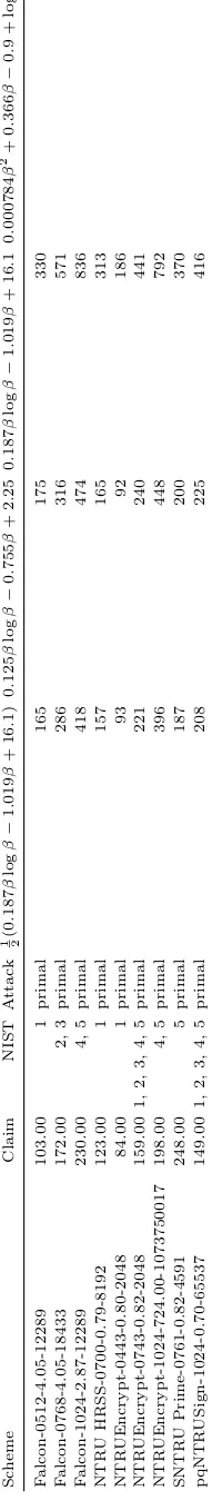
Our results are given in Tables 5, 6, 7, 8, 9, and 10 in Appendix A. In

addi-tion, we make available at

https://estimate-all-the-lwe-ntru-schemes.

github.io

a human-friendly version of these tables. In particular, the

HTML version supports filtering and sorting the table. It also contains

SageMath source code snippets to reproduce each entry. As discussed

above, the meaning of the output values vary depending on cost model

since the unit of computation is not consistent across different cost models.

Furthermore, submissions might consider different units of computation,

such as bit security, even when using a particular cost model. Furthermore,

we do not consider memory requirements in this work.

In the following, we illuminate some of the choices and assumptions we

made to arrive at our estimates.

Secret distributions.

The majority of the submissions consider

uni-form, bounded uniuni-form, or sparse bounded uniform secret distributions.

In the case of Lizard, LWE secrets are drawn from the distribution

ZO

(

ρ

) for some 0

< ρ <

1.

ZO

(

ρ

) is the distribution over

{−

1

,

0

,

1

}

where each component

si

(of a vector

s

← ZO

(

ρ

)) satisfies Pr [

si

= 1] =

Pr [

s

=

−

1] =

ρ/

2 and Pr [

s

= 0] = 1

−

ρ

. We model this distribution as

a fixed weight bounded uniform distribution, where the Hamming weight

h

matches the expected number of non-zero components of an element

drawn from

ZO

(

ρ

).

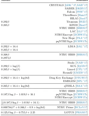
5

Model

Schemes

CRYSTALS [LDK

17,SAB

17]

SABER [DKRV17]

Falcon [PFH

17]

ThreeBears [Ham17]

HILA5 [Saa17]

0

.

292

β

Titanium [SSZ17]

0

.

265

β

KINDI [Ban17]

NTRU HRSS [SHRS17]

LAC [LLJ

17]

NTRUEncrypt [ZCHW17a]

New Hope [PAA

_17]

pqNTRUSign [ZCHW17b]

0

.

292

β

+ 16

.

4

LIMA [SAL

_17]

0

.

265

β

+ 16

.

4

0

.

368

β

NTRU HRSS [SHRS17]

0

.

2975

β

Frodo [NAB

17]

0

.

292

β

+ log(

β

)

KCL [ZjGS17]

0

.

265

β

+ log(

β

)

Lizard [CPL

17]

Round2 [GMZB

17]

0

.

292

β

+ 16

.

4 + log(8

d

)

Ding Key Exchange [DTGW17]

EMBLEM [SPL

17]

0

.

265

β

+ 16

.

4 + log(8

d

)

qTESLA [BAA

17]

NTRU HRSS [SHRS17]

0

.

187

β

log

β

−

1

.

019

β

+ 16

.

1

pqNTRUSign [ZCHW17b]

NTRUEncrypt [ZCHW17a]

1

2

(0

.

187

β

log

β

−

1

.

019

β

+ 16

.

1)

NTRU HRSS [SHRS17]

0

.

000784

β

+ 0

.

366

β

−

0

.

9 + log(8

d

)

NTRU Prime [BCLvV17]

0

.

125

β

log

β

−

0

.

755

β

+ 2

.

25

LOTUS [PHAM17]

Error distributions.

While the estimator assumes the distribution of

error vector components to be a discrete Gaussian, many submissions

use alternatives. Binomial distributions are treated as discrete Gaussians

with the corresponding standard deviation. Similarly, bounded uniform

distributions

U

are also treated as discrete Gaussians with standard

deviation,

q

V

[

U

]. In the case of LWR, we use a standard deviation of

q

(q/p)2−1

12

, following [Ngu18].

Success probability.

The estimator supports defining a target success

probability for both the primal and dual attack. The only proposal we

found that explicitly uses this functionality is LIMA [SAL

_{17], which}

chooses to use a target success probability of 51%. For our estimates we

imposed this to be the estimator’s default 99% for all schemes, since it

seems to make little to no difference for the final estimates as amplification

in this range is rather cheap.

Known limitations.

While the estimator can scale short secret vectors

with entries sampled from a bounded uniform distribution, it does not

attempt to shift secret vectors whose entries have unbalanced bounds to

optimise the scaling. Similarly, it does not attempt to guess entries of such

secrets to use a hybrid combinatorial approach. We note, however, that

only the KINDI submission [Ban17] uses such a secret vector distribution.

In this case, the deviation from a distribution centred at zero is small and

we thus ignore it.

NTRU.

For estimating NTRU-based schemes, we also utilise the LWE

estimator as described here to evaluate the primal attack (and its

im-provements, when considered in combination with dimension reduction)

on NTRU. In particular, we cost NTRU as a uSVP instance but note

that when no guessing is performed, the geometry of the NTRU-lattice

can possibly be exploited as in [KF17]. The dual attack is not considered,

as it does not apply. Let (

f

,

g

)

∈

Z

be the secret NTRU vector. We

modulus. The secret distribution is set to the distribution of

f

. We limit

the number of LWE samples to

n

. The estimator is set to consider the

n

rotations of

g

when estimating the cost of the primal attack on NTRU.

Beyond key recovery.

We consider key recovery attacks on all schemes.

In the case of LWE-based schemes, we also consider message recovery

attacks by setting the number of samples to be

m

= 2

n

and trying to

recover the ephemeral secret key set as part of key encapsulation. A

straightforward primal uSVP message recovery attack for NTRU-based

schemes as described in Footnote 2 of [SHRS17] is not expected to perform

better than the primal uSVP key recovery attack, and is therefore omitted

in this work.

In the case of signatures, it is also possible to attempt forgery attacks.

All four lattice-based signatures schemes submitted to the NIST process

claim that the problem of forging a signature is strictly harder than that

of recovering the signing key. In particular Dilithium and pqNTRUSign

provide analyses which explicitly determine that larger BKZ block sizes

are required for signature forgery than key recovery. Falcon argues

sim-ilarly without giving explicit block sizes and qTESLA presents a tight

reduction in the QROM from the RLWE problem to signature forgery,

in particular from exactly the RLWE problem one would have to solve

to yield the signing key. As such, since one may trivially forge signatures

given possession of the signing key, forgery attacks are not considered

further in their security analyses.

6

Discussion

Our data highlights that cost models for lattice reduction do not necessarily

preserve the ordering of the schemes under consideration. That is, under

one cost model some scheme A can be considered harder to break than a

scheme B, while under another cost model scheme B appears harder to

break.

An example for the schemes EMBLEM and uRound2.KEM was highlighted

in [Ber18]. Specifically, the example concerns the EMBLEM parameter

set with

n

= 611 and the uRound2.KEM parameter set with

n

= 500. In

the 0

.

292

β

cost model, the cost of the primal attack for EMBLEM-611 is

estimated as

76 and for uRound2.KEM-500 as 84. For the same attack

in the 0

.

187

β

log

β

−

1

.

019

β

+ 16

.

1 cost model, the cost is estimated for

EMBLEM-611 as 142 and for uRound2.KEM-500 as 126. Similar swaps

can be observed for several other pairs of schemes and cost models. In

most cases the estimated securities of the two schemes are very close to

each other (differing by, say, 1 or 2) and thus a swap of ordering does

not fundamentally alter our understanding of their relative security as

these estimates are typically derived by heuristically searching through

the space of possible parameters and computing with limited precision. In

some cases, though, such as the one highlighted in [Ber18], the differences

in security estimates can be significant. There are two classes of such

cases.

Sparse secrets.

The first class of cases involves instances with sparse

secrets. The LWE estimator applies guessing strategies when costing the

dual attack (cf. [Alb17]) and the primal attack. The basic idea is that

for a sparse secret, many of the entries of the secret vector are zero,

and hence can be ignored. We guess

τ

entries to be zero, and drop the

corresponding columns from the attack lattice. In dropping

τ

columns

from a

n

-dimensional LWE instance, we obtain a (

n

−

τ

)-dimensional LWE

instance with a more dense secret distribution, where the density depends

on the choice of

τ

and the original value of

h

. On the one hand, there is a

probability of failure when guessing which columns to drop. On the other

hand there may exist a

τ

for which the (

n

−

τ

)-dimensional LWE instance

is easier to solve, and in particular requires a smaller BKZ blocksize

β

.

6

The trade-off between running BKZ on smaller lattices and having to

run it multiple times can correspond to an overall lower expected attack

cost. This probability of failure when guessing secret entries does not

depend on the cost model, but rather on the weight and dimension of the

secret, making this kind of attack more effective for very sparse secrets.

In the case of comparing an enumeration cost model versus a sieving

one, we have that the cost of enumeration is fitted as 2

or 2

whereas the cost of sieving is 2

. The steeper curve for enumeration

means that as we increase

τ

, and hence decrease

β

, savings are potentially

larger, justifying a larger number

τ

of entries guessed. Concretely, the

computed optimal guessing dimension

τ

can be much larger than in the

sieving regime. This phenomenon can also be observed when comparing

two different sieving models or two different enumeration models.

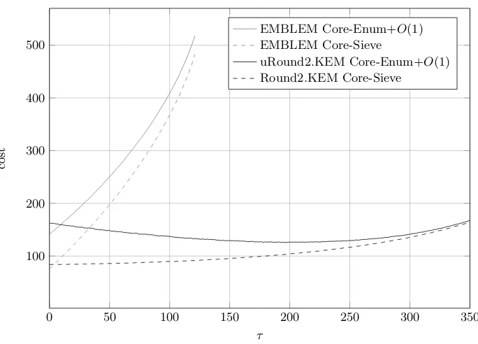
In Figure 1, we illustrate this for the EMBLEM and uRound2.KEM

example. EMBLEM does not have a sparse secret, while uRound2.KEM

does. For EMBLEM the best guessing dimension, giving the lowest overall

cost, is

τ

= 0 in both cost models. For uRound2.KEM, we see that the

optimal guessing dimension varies depending on the cost model. In the

0

.

292

β

cost model, the lowest overall expected cost is achieved for

τ

= 1

while in the 0

.

187

β

log

β

−

1

.

019

β

+ 16

.

1 model the optimal choice is

τ

= 197.

Dual attack.

The second class of cases can be observed for the dual attack.

Recall that the dual attack runs lattice reduction to find a small vector

v

in

the scaled dual lattice of

A

and then considers

h

v

,

b

i

which is short when

A

,

b

is an LWE sample. In more detail, the advantage of distinguishing

h

v

,

b

i

is

ε

= exp(

−

δ

·

c

) for some constant

c

depending on the instance

and with

d

being the dimension of the lattice under consideration [LP11].

To amplify this advantage to a constant advantage, we have to repeat

the experiment roughly 1

/ε

times. Thus, the overall cost of the attack is

≈

C

(

β

)

/

exp(

−

δ

·

c

)

2

where

C

(

β

) is the cost of lattice reduction with

block size

β

. In the sieving regime

C

(

β

)

≈

2

_{in the enumeration regime}

we have

C

(

β

)

≈

β

(from enumeration costing 2

). For large

β

we have

δ

≈

β

[Che13] (cf. Section 2), and thus we have overall log

costs of roughly

c

β

+ 2 log(

e

)

β

c

resp.

c

β

log(

β

) + 2 log(

e

)

β

c

.

0

50

100

150

200

250

300

350

100

200

300

400

500

τ

cost

EMBLEM Core-Enum+

O

(1)

EMBLEM Core-Sieve

uRound2.KEM Core-Enum+

O

(1)

Round2.KEM Core-Sieve

Fig. 1.

Estimates of the cost of the primal attack when guessing

τ

secret entries for the

schemes EMBLEM-611 and uRound2.KEM-500 using cost models Core-Enum+

O

(1)

and Core-Sieve.

optimal

β

in the sieving regime is not necessarily the optimal

β

in the

enumeration regime.

We stress that while the above discussion gives an account of why our

esti-mates show the behaviour we observe, it leaves the fundamental question

partially unanswered: how does the security of the schemes considered

in this work compare to one another. As it stands, the answer to this

question depends on which between enumeration and sieving is the

correct

regime to consider for a given block size, i.e. from which dimension sieving

beats enumeration. Thus, resolving this question is a pressing concern.

LWE problem), and there are also parameter sets for which the converse

is true. To deal with this issue, for each parameter set, in each cost model,

for each attack, we always choose the lower of the two possible costs.

Quantum security.

In [Nat16], NIST defines five security categories

that schemes should target in the presence of an adversary with access to

a quantum computing device. They furthermore propose as a plausible

assumption that such a device would support a maximum quantum circuit

depth

MAXDEPTH

≤

2

(although they do not mention a preferred set of

universal gates to consider). Since concrete designs for large scale quantum

computers are still an open research problem, not all schemes take this

limitation into account, and many opt for using a (quantum) asymptotic

cost model that considers the best known theoretical Grover speed-up,

resulting in overestimates of the adversary’s power.

This use of quantum cost models introduces a further difficulty when

trying to compare schemes based on the outputs of the [APS15] estimator.

For example, the security definition of Category 1 says that attacks on

schemes should be as hard as AES128 key recovery. Some schemes address

this by tuning their parameters to match hardness (using a quantum cost

model)

≥

2

, in the vein of “128 bit security”. On the other hand, other

schemes claiming the same category match hardness (using a quantum

cost model)

≥

2

since key recovery on AES128 can be considered as

a search problem in an unstructured list of size 2

, which Grover can

complete in

O

(2

) time. This results in schemes with rather different

cycle counts and memory usage claiming the same security category, as

can be seen from the “claimed security” column in the estimates table.

Acknowledgements

References

ACFP14.

Martin R. Albrecht, Carlos Cid, Jean-Charles Faug`

ere, and Ludovic

Per-ret. Algebraic algorithms for LWE. Cryptology ePrint Archive, Report

2014/1018, 2014.

http://eprint.iacr.org/2014/1018

.

ACPS09.

Benny Applebaum, David Cash, Chris Peikert, and Amit Sahai. Fast

cryptographic primitives and circular-secure encryption based on hard

learning problems. In Shai Halevi, editor,

CRYPTO 2009

, volume 5677 of

LNCS

, pages 595–618. Springer, Heidelberg, August 2009.

ADPS16.

Erdem Alkim, L´

eo Ducas, Thomas P¨

oppelmann, and Peter Schwabe.

Post-quantum key exchange - A new hope. In Thorsten Holz and Stefan Savage,

editors,

25th USENIX Security Symposium, USENIX Security 16

, pages

327–343. USENIX Association, 2016.

AFFP14.

Martin R. Albrecht, Jean-Charles Faug`

ere, Robert Fitzpatrick, and Ludovic

Perret. Lazy modulus switching for the BKW algorithm on LWE. In

Hugo Krawczyk, editor,

PKC 2014

, volume 8383 of

LNCS

, pages 429–445.

Springer, Heidelberg, March 2014.

AG11.

Sanjeev Arora and Rong Ge. New algorithms for learning in presence of

errors. In Luca Aceto, Monika Henzinger, and Jiri Sgall, editors,

ICALP

2011, Part I

, volume 6755 of

LNCS

, pages 403–415. Springer, Heidelberg,

July 2011.

AGVW17.

Martin R. Albrecht, Florian G¨

opfert, Fernando Virdia, and Thomas

Wun-derer. Revisiting the expected cost of solving uSVP and applications to

LWE. In Tsuyoshi Takagi and Thomas Peyrin, editors,

ASIACRYPT 2017,

Part I

, volume 10624 of

LNCS

, pages 297–322. Springer, Heidelberg,

De-cember 2017.

Ajt96.

Mikl´

os Ajtai. Generating hard instances of lattice problems (extended

abstract). In

28th ACM STOC

, pages 99–108. ACM Press, May 1996.

AKS01.

Mikl´

os Ajtai, Ravi Kumar, and D. Sivakumar. A sieve algorithm for the

shortest lattice vector problem. In

33rd ACM STOC

, pages 601–610. ACM

Press, July 2001.

Alb17.

Martin R. Albrecht. On dual lattice attacks against small-secret LWE

and parameter choices in HElib and SEAL. In Jean-S´

ebastien Coron and

Jesper Buus Nielsen, editors,

EUROCRYPT 2017, Part II

, volume 10211

of

LNCS

, pages 103–129. Springer, Heidelberg, April / May 2017.

APS15.

Martin R Albrecht, Rachel Player, and Sam Scott. On the concrete hardness

of Learning with Errors.

Journal of Mathematical Cryptology

, 9(3):169–203,

2015.

BAA

17.

Nina Bindel, Sedat Akleylek, Erdem Alkim, Paulo S. L. M. Barreto,

Johannes Buchmann, Edward Eaton, Gus Gutoski, Juliane Kramer,

Patrick Longa, Harun Polat, Jefferson E. Ricardini, and Gustavo

Zanon.

qtesla.

Technical report, National Institute of Standards

and Technology, 2017. available at

https://csrc.nist.gov/projects/

post-quantum-cryptography/round-1-submissions

.

Ban17.

Rachid El Bansarkhani. Kindi. Technical report, National Institute of

Standards and Technology, 2017. available at

https://csrc.nist.gov/

projects/post-quantum-cryptography/round-1-submissions

.

BDGL16.

Anja Becker, L´

eo Ducas, Nicolas Gama, and Thijs Laarhoven. New

di-rections in nearest neighbor searching with applications to lattice sieving.

In Robert Krauthgamer, editor,

27th SODA

, pages 10–24. ACM-SIAM,

January 2016.

Ber17.

Daniel J. Bernstein.

Table of ciphertext and key sizes for the NIST

candidate algorithms. Available at

https://groups.google.com/a/list.

nist.gov/d/msg/pqc-forum/1lDNio0sKq4/xjqy4K6SAgAJ

, 2017.

Ber18.

Daniel J. Bernstein, 2018. Comment on PQC forum in response to an

earlier version of this work. Available at

https://groups.google.com/a/

list.nist.gov/d/msg/pqc-forum/h4_LCVNejCI/FyV5hgnqBAAJ

.

BG14.

Shi Bai and Steven D. Galbraith. Lattice decoding attacks on binary LWE.

In Willy Susilo and Yi Mu, editors,

ACISP 14

, volume 8544 of

LNCS

,

pages 322–337. Springer, Heidelberg, July 2014.

Che13.

Yuanmi Chen.

R´

eduction de r´

eseau et s´

ecurit´

e concr`

ete du chiffrement

compl`

etement homomorphe

. PhD thesis, Paris 7, 2013.

CHK

17.

Jung Hee Cheon, Kyoohyung Han, Jinsu Kim, Changmin Lee, and Yongha

Son. A practical post-quantum public-key cryptosystem based on

spLWE

.

In Seokhie Hong and Jong Hwan Park, editors,

ICISC 16

, volume 10157

of

LNCS

, pages 51–74. Springer, Heidelberg, November / December 2017.

CN11.

Yuanmi Chen and Phong Q. Nguyen. BKZ 2.0: Better lattice security

esti-mates. In Dong Hoon Lee and Xiaoyun Wang, editors,

ASIACRYPT 2011

,

volume 7073 of

LNCS

, pages 1–20. Springer, Heidelberg, December 2011.

CPL

17.

Jung Hee Cheon, Sangjoon Park, Joohee Lee, Duhyeong Kim, Yongsoo

Song, Seungwan Hong, Dongwoo Kim, Jinsu Kim, Seong-Min Hong, Aaram

Yun, Jeongsu Kim, Haeryong Park, Eunyoung Choi, Kimoon kim,

Jun-Sub Kim, and Jieun Lee. Lizard. Technical report, National Institute of

Standards and Technology, 2017. available at

https://csrc.nist.gov/

projects/post-quantum-cryptography/round-1-submissions

.

CS97.

Don Coppersmith and Adi Shamir. Lattice attacks on NTRU. In

Wal-ter Fumy, editor,

EUROCRYPT’97

, volume 1233 of

LNCS

, pages 52–61.

Springer, Heidelberg, May 1997.

DKRV17.

Jan-Pieter D’Anvers, Angshuman Karmakar, Sujoy Sinha Roy, and Frederik

Vercauteren. Saber. Technical report, National Institute of Standards

and Technology, 2017. available at

https://csrc.nist.gov/projects/

post-quantum-cryptography/round-1-submissions

.

DT17.

Fplll Development Team. fplll, a lattice reduction library. Available at

https://github.com/fplll/fplll

, 2017.

DTGW17.

Jintai Ding, Tsuyoshi Takagi, Xinwei Gao, and Yuntao Wang.

Ding

key exchange.

Technical report, National Institute of Standards

and Technology, 2017. available at

https://csrc.nist.gov/projects/

post-quantum-cryptography/round-1-submissions

.

FP85.

U. Fincke and M. Pohst. Improved methods for calculating vectors of

short length in a lattice, including a complexity analysis.

Mathematics of

Computation

, 44(170):463–463, May 1985.

Fuj17.

Ryo Fujita. Table of underlying problems of the NIST candidate

algo-rithms. Available at

https://groups.google.com/a/list.nist.gov/d/

msg/pqc-forum/1lDNio0sKq4/7zXvtfdZBQAJ

, 2017.

GJMS17.

Qian Guo, Thomas Johansson, Erik M˚

artensson, and Paul Stankovski.

Coded-BKW with sieving. In Tsuyoshi Takagi and Thomas Peyrin, editors,

GJS15.

Qian Guo, Thomas Johansson, and Paul Stankovski. Coded-BKW: Solving

LWE using lattice codes. In Rosario Gennaro and Matthew J. B.

Rob-shaw, editors,

CRYPTO 2015, Part I

, volume 9215 of

LNCS

, pages 23–42.

Springer, Heidelberg, August 2015.

GMZB

_{17. Oscar Garcia-Morchon, Zhenfei Zhang, Sauvik Bhattacharya, Ronald}

Rietman, Ludo Tolhuizen, and Jose-Luis Torre-Arce. Round2. Technical

report, National Institute of Standards and Technology, 2017. available

at

https://csrc.nist.gov/projects/post-quantum-cryptography/

round-1-submissions

.

GN08.

Nicolas Gama and Phong Q. Nguyen. Finding short lattice vectors within

Mordell’s inequality. In Richard E. Ladner and Cynthia Dwork, editors,

40th ACM STOC

, pages 207–216. ACM Press, May 2008.

Gro96.

Lov K. Grover. A fast quantum mechanical algorithm for database search.

In

28th ACM STOC

, pages 212–219. ACM Press, May 1996.

Ham17.

Mike Hamburg. Three bears. Technical report, National Institute of

Standards and Technology, 2017. available at

https://csrc.nist.gov/

projects/post-quantum-cryptography/round-1-submissions

.

HG07.

Nick Howgrave-Graham. A hybrid lattice-reduction and meet-in-the-middle

attack against NTRU. In Alfred Menezes, editor,

CRYPTO 2007

, volume

4622 of

LNCS

, pages 150–169. Springer, Heidelberg, August 2007.

HPS96.

Jeffery Hoffstein, Jill Pipher, and Joseph H. Silverman. NTRU: A new

high speed public-key cryptosystem. Technical report, Draft distributed

at CRYPTO96, 1996. available at

https://cdn2.hubspot.net/hubfs/

49125/downloads/ntru-orig.pdf

.

HPS98.

Jeffrey Hoffstein, Jill Pipher, and Joseph H. Silverman. NTRU: A

ring-based public key cryptosystem. In

Algorithmic Number Theory, Third

International Symposium, ANTS-III, Portland, Oregon, USA, June 21-25,

1998, Proceedings

, pages 267–288, 1998.

HPS

15.

Jeff Hoffstein, Jill Pipher, John M. Schanck, Joseph H. Silverman, William

Whyte, and Zhenfei Zhang.

Choosing parameters for NTRUEncrypt.

Cryptology ePrint Archive, Report 2015/708, 2015.

http://eprint.iacr.

org/2015/708

.

Kan83.

Ravi Kannan. Improved algorithms for integer programming and related

lattice problems. In

15th ACM STOC

, pages 193–206. ACM Press, April

1983.

Kan87.

Ravi Kannan. Minkowski’s convex body theorem and integer programming.

Mathematics of Operations Research

, pages 415–440, 1987.

KF15.

Paul Kirchner and Pierre-Alain Fouque. An improved BKW algorithm for

LWE with applications to cryptography and lattices. In Rosario Gennaro

and Matthew J. B. Robshaw, editors,

CRYPTO 2015, Part I

, volume 9215

of

LNCS

, pages 43–62. Springer, Heidelberg, August 2015.

KF17.

Paul Kirchner and Pierre-Alain Fouque. Revisiting lattice attacks on

overstretched NTRU parameters. In Jean-S´

ebastien Coron and Jesper Buus

Nielsen, editors,

EUROCRYPT 2017, Part I

, volume 10210 of

LNCS

, pages

3–26. Springer, Heidelberg, April / May 2017.

Laa15a.

Thijs Laarhoven.

Search problems in cryptography: From fingerprinting to

lattice sieving

. PhD thesis, Eindhoven University of Technology, 2015.

Laa15b.

Thijs Laarhoven. Sieving for shortest vectors in lattices using angular

LDK

17.

Vadim Lyubashevsky, Leo Ducas, Eike Kiltz, Tancrede Lepoint,

Peter

Schwabe,

Gregor

Seiler,

and

Damien

Stehle.

Crystals-dilithium.

Technical report, National Institute of Standards and

Technology, 2017.

available at

https://csrc.nist.gov/projects/

post-quantum-cryptography/round-1-submissions

.

LLJ

17.

Xianhui Lu, Yamin Liu, Dingding Jia, Haiyang Xue, Jingnan He, and

Zhenfei Zhang. Lac. Technical report, National Institute of Standards

and Technology, 2017. available at

https://csrc.nist.gov/projects/

post-quantum-cryptography/round-1-submissions

.

LMvdP15.

Thijs Laarhoven, Michele Mosca, and Joop van de Pol. Finding shortest

lat-tice vectors faster using quantum search.

Designs, Codes and Cryptography

,

77(2–3):375–400, December 2015.

LP11.

Richard Lindner and Chris Peikert. Better key sizes (and attacks) for

LWE-based encryption. In Aggelos Kiayias, editor,

CT-RSA 2011

, volume

6558 of

LNCS

, pages 319–339. Springer, Heidelberg, February 2011.

LPR10.

Vadim Lyubashevsky, Chris Peikert, and Oded Regev. On ideal lattices

and learning with errors over rings. In Henri Gilbert, editor,

EURO-CRYPT 2010

, volume 6110 of

LNCS

, pages 1–23. Springer, Heidelberg,

May / June 2010.

LS15.

Adeline Langlois and Damien Stehl´

e. Worst-case to average-case reductions

for module lattices.

Designs, Codes and Cryptography

, 75(3):565–599, June

2015.

Moo17.

Dustin Moody.

The NIST post quantum cryptography

“competi-tion”.

Available at

https://csrc.nist.gov/CSRC/media/Projects/

Post-Quantum-Cryptography/documents/asiacrypt-2017-moody-pqc.

pdf

, 2017.

MR09.

Daniele Micciancio and Oded Regev. Lattice-based cryptography. In

Daniel J. Bernstein, Johannes Buchmann, and Erik Dahmen, editors,

Post-Quantum Cryptography

, pages 147–191. Springer, Heidelberg, Berlin,

Heidelberg, New York, 2009.

MS01.

Alexander May and Joseph H. Silverman. Dimension reduction methods for

convolution modular lattices. In

Cryptography and Lattices, International

Conference, CaLC 2001, Providence, RI, USA, March 29-30, 2001, Revised

Papers

, pages 110–125, 2001.

MW15.

Daniele Micciancio and Michael Walter. Fast lattice point enumeration

with minimal overhead. In Piotr Indyk, editor,

26th SODA

, pages 276–294.

ACM-SIAM, January 2015.

NAB

17.

Michael Naehrig, Erdem Alkim, Joppe Bos, Leo Ducas, Karen

Easter-brook, Brian LaMacchia, Patrick Longa, Ilya Mironov, Valeria

Niko-laenko, Christopher Peikert, Ananth Raghunathan, and Douglas

Ste-bila.

Frodokem.

Technical report, National Institute of Standards

and Technology, 2017. available at

https://csrc.nist.gov/projects/

post-quantum-cryptography/round-1-submissions

.

Nat16.

National Institute of Standards and Technology. Submission requirements

and evaluation criteria for the Post-Quantum Cryptography

standardiza-tion process.

http://csrc.nist.gov/groups/ST/post-quantum-crypto/

documents/call-for-proposals-final-dec-2016.pdf

, December 2016.

Nat17.

National Institute of Standards and Technology. Performance testing of