Modified PSO Algorithm for Real-time Energy Management in
Grid-connected Microgrids
Md Alamgir Hossain1,2,∗, Hemanshu Roy Pota1, Stefano Squartini3 and Ahmed Fathi Abdou1
1School of Engineering & Information Technology, The University of New South Wales, Canberra, ACT 2610, Australia
2Department of Electrical & Electronic Engineering, Dhaka University of Engineering and Technology, Gazipur, Bangladesh
3Department of Information Engineering, Universit`aPolitecnica delle Marche, Ancona, Italy
Abstract
Real-time energy management of a converter-based microgrid is difficult to determine optimal operating
points of a storage system in order to save costs and minimise energy waste. This complexity arises due to
time-varying electricity prices, stochastic energy sources and power demand. Many countries have imposed
real-time electricity pricing to efficiently control demand side management. This paper presents a particle
swarm optimisation (PSO) for the application of real-time energy management to find optimal battery controls
of a community microgrid. The modification of the PSO consists in altering the cost function to better model
the battery charging/discharging operations. As optimal control is performed by formulating a cost function, it
is suitably analysed and then a dynamic penalty function in order to obtain the best cost function is proposed.
Several case studies with different scenarios are conducted to determine the effectiveness of the proposed cost
function. The proposed cost function can reduce operational cost by 12% as compared to the original cost
function over a time horizon of 96 hours. Simulation results reveal the suitability of applying the regularised
PSO algorithm with the proposed cost function, which can be adjusted according to the need of the community,
for real-time energy management.
Keywords: Converter-based microgrids, renewable energy sources, optimum battery control, real-time energy
management, and particle swarm optimisation.
Abbreviations
The following abbreviations are used in this manuscript:
PSO Particle swarm optimisation
RESs Renewable energy sources
ESS Energy storage system
SOC State of charge
ADP Adaptive dynamic programming
I-DEMS Intelligent dynamic energy management system
PV Photovoltaic
PCC Point of common-coupling
EMS Energy management system
BLo Initial battery energy level
BLmax Maximum battery energy level
BLmin Minimum battery energy level
PwT Total wind power
PsT Total solar power
Pg Import/export grid power
L(t) Load at timet
5
∗Corresponding author
Cost Objective function
u Battery command signals
fpc(C) Penalty cost function
RRTP Real-time residential electricity price
WT Wind turbine
SI Solar irradiation
Pc,max Maximum charging rate
Pd,max Maximum discharging rate
η Efficiency
CF Constriction factor
φ Constriction co-efficient
1. Introduction
The penetration of intermittent renewable energy sources (RESs), such as wind and solar, into existing
distribution networks has increased significantly to meet the growing electricity demand and fulfil the target
of reducing greenhouse gas emissions [1, 2]. However, these RESs, depending on weather conditions and time
10
of day, are stochastic in nature, resulting in variable power generation. Random application of RESs with this
intermittent power generation can create difficulty in control, operation and management of the distribution
network [3]. To minimise complexities on an existing power system, the concept of a microgrid has been
introduced [4]. A microgrid (consisting of small-scale emerging generators, loads, energy storage elements
and a control unit) is a controlled, small-scale power system that can be operated in an islanded and/or
15
grid-connected mode in a defined area to facilitate the provision of supplementary power and/or maintain a
standard service [5]. In the case of grid-tied microgrids, power can be exchanged with the main grid depending
on electricity prices. Although electricity price per kWh is generally fixed, it may vary over the time to have
better demand management with the help of smart meter technologies capable of measuring power generation
and demand in each time instant [6].
20
The central control unit in a microgrid is responsible for efficient power management with the help of
an energy storage system (ESS) during the operation of the grid-following or grid-forming mode [7]. The
application of ESSs increases the stability of the grid utility, upgrades the capacity of transmission lines, allows
RES penetration, levels load curves, mitigates voltage fluctuation, and improves power quality and reliability
[8]. An ESS absorbs surplus power and then dispatches it later when input sources are not available, e.g., at
25
night time for solar PV panels. In addition, energy can be stored when electricity prices are low and sold during
the hours of high prices to minimise operational costs, allowing more flexible and reliable energy management
for a community microgrid. To control the battery energy optimally for reducing electricity costs of investors,
the formulation of the cost function considering charging and discharging factors needs to be carefully analysed
in addition to the application of efficient algorithms.
30
An intelligent energy management for handling uncertainties in microgrids becomes essential to maintain
a reliable power supply. Energy management for a microgrid, consisting of solar, wind and battery, involves
determining the most economical control of stored energy that reduces operating costs subject to the satisfaction
of a number of operating constraints. Although conventional if-else rule-based policies, where initial sets of
rules are fixed for different scenarios, are employed, they can not provide an optimal control policy [9, 10].
35
Generally, in this method, energy is dispatched based on available power and state of charge (SOC) of the
battery, and stored if power generation is higher than power demand [11]. In addition, abrupt charging and
To improve optimal control approaches for battery energy, a lot of optimisation algorithms, such as linear
programming [12, 13, 14], dynamic programming [15], fuzzy logic [16] and adaptive dynamic control [17],
40
are presented in literature. In [18], an expert-based control approach incorporating operating constraints,
such as SOC limits and charging/discharging current limits, is presented to optimally use the storage systems
for dispatching RESs smoothly. In [16], a fuzzy logic expert system to minimise the operations cost and
emission levels of a microgrid is developed. A power management mechanism using dynamic programming for
photovoltaic (PV) systems with storage to allow massive penetration of PV power into a distribution network
45
is described in [19]. In [20], a firefly algorithm to find the optimal operation of a microgrid considering lifetime
characteristics of a battery is applied. A batch reinforcement learning algorithm to optimally schedule the
battery energy for maximising the self-consumption of the local power generation in a microgrid is presented
in [21]. The adaptive dynamic programming (ADP) for the residential power management and control that
focuses on a home battery management is applied in [22]. ADP is employed in an office building to control
50
battery energy management optimally [23]. An intelligent dynamic energy management system (I-DEMS) is
developed to optimally use RESs and an energy storage system for maintaining continuous electricity supply
to critical loads [9].
In most of the literature reported above, the contribution remains in the application of new algorithms
with different objective functions and reduction of simulation time to minimise operational costs. Although a
55
formulation of an objective function has a direct involvement in altering results, little attention has been paid
when applying it to efficiently control the battery energy. Consequently, slight improvements in their results
can be observed when their methods are compared to that of others. To find improved solutions quickly and
continuously, this paper proposes a particle swarm optimisation (PSO) that runs any time a new sample is
available (in our simulations this occurs with a sampling time equal to 1 h) for analysing cost functions and
60
then a penalty function related to a dynamic electricity price is multiplied to the charging component. This
is done for optimally charging and discharging the battery energy in order to exchange energy with the grid
utility depending on electricity prices and availability of local power generated. The major contributions are
listed as follows:
• A regularised PSO algorithm in which a different procedure from the conventional one is presented for
65
the application of real-time energy management for a community microgrid;
• Cost functions, used to determine the output of an optimisation algorithm, for determining
charg-ing/discharging energy amount of a battery are analysed; and
• A dynamic penalty function, which can be tuned, depending on energy generation from RESs, to efficiently
manage battery energy is proposed to the cost function.
70
The rest of the paper is organised as follows. Section 2 introduces an overview of a community microgrid. In
Section 3, the different components of the microgrid to facilitate the analysis are modelled. Section 4 proposes a
cost function with constraints after analysing other cost functions. In Section 5, the metaheuristic optimisation
algorithm in the standard and regularised forms is presented. Simulation results for the different cost functions
in two scenarios are performed in Section 6. Section 7 concludes the study.
ESS
Grid
400 V
20 kV
PV
PV
PV
WT
WT
WT
EMS
PCC
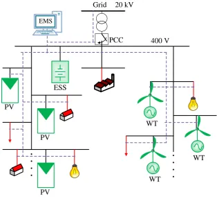
Figure 1: Typical converter-based microgrid.
2. Description of a community microgrid
A community microgrid using local resources to meet power demand is illustrated in Figure 1. The
com-munity, consisting of twenty houses, has five solar generators (4 kW) and six wind generators (5 kW) installed.
Thus, the microgrid consists of PV generators, wind generators, an energy storage system, local loads, a main
electrical grid and an energy management system (EMS). It is connected to the main grid through a transformer
80
and the point of common coupling (PCC). Although the microgrid is capable of operating either islanded or
grid-tied modes, only the latter is taken into account for this paper to exchange powers. The main grid and
RESs can supply the power to loads and/or charge the battery. The excess energy after fulfilling local demands
from RESs can be sold to the grid in order to reduce operational costs. Due to security and reliability issues of
continuous power supply to local loads, in this study, the battery energy is not sold.
85
The EMS manages energy to ensure the requirement of the local power demand over the time periods and
to exchange power with the main grid during the excess and scarcity of the local power generation. Although a
number of countries may not approve an energy business with the grid utility due to their rules and regulations,
this study considers case studies where there are no obligations for this business rather than an encouragement
for microgrid investors. The total capacity for PV generators, wind generators and battery are taken as 20 kW,
90
30 kW and 35 kWh, respectively. The battery capacity, considered to supply for one hour local load, increases
complexities of the analysis due to a small storage system with stochastic power generation. Generally, battery
capacity is estimated three times greater than the maximum load demand to maintain continuous supply at least
three hours after the loss of grid connection [24]. The optimal size determination of the microgrid parameters
is beyond the scope of this paper. The parameters of the solar generator, wind generator and battery are given
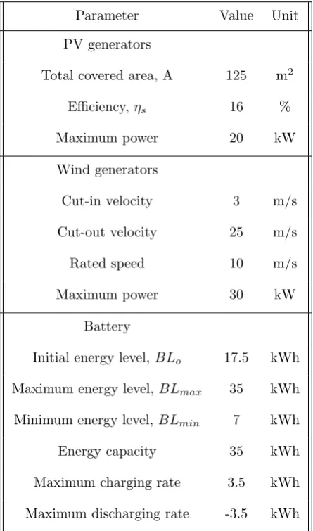
Table 1: Input parameters.
Parameter Value Unit
PV generators
Total covered area, A 125 m2
Efficiency,ηs 16 %
Maximum power 20 kW
Wind generators
Cut-in velocity 3 m/s
Cut-out velocity 25 m/s
Rated speed 10 m/s
Maximum power 30 kW
Battery
Initial energy level, BLo 17.5 kWh
Maximum energy level,BLmax 35 kWh
Minimum energy level,BLmin 7 kWh
Energy capacity 35 kWh
Maximum charging rate 3.5 kWh
Maximum discharging rate -3.5 kWh
in Table 1.
Although generated power, which is unpredictable and can not directly be handled, may be partially
con-trolled using power curtailment strategy, this study considers operating all RESs in maximum power tracking
modes to extract maximum power. As a result, controlling battery energy, which is a crucial issue for the
con-sideration of dynamic electricity prices, available energy and satisfaction of power demand, is the only option
100
for these types of microgrids. The battery can only be operated as one of the following modes at a time:
• Charge modes: the battery can be charged from the grid and/or RESs with an energy quantity which
is not beyond the charging rate;
• Discharge modes: the battery supplies energy to loads when prices are high with an energy quantity
within the battery discharging rate;
105
• Inactive modes: there is no activity of the battery energy in this mode as the grid utility directly supplies
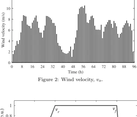
0 8 16 24 32 40 48 56 64 72 80 88 96
Time (h)
0 2 4 6 8 10 12
Wind velocity (m/s)
Figure 2: Wind velocity,vo.
Figure 3: Power curve of wind generator.
3. System modeling
3.1. Wind generators
Wind power, a free available energy source, is the electric power generated by rotating turbine blades,
mounted on a tower at a considerable height, while wind hits the blades of the wind turbine. As wind is
stochastic in nature, wind turbines have no control over its generated power. Therefore, power generation by
wind turbines solely depends on the availability of wind speed and this varies with heights. The wind speed v1
is shown in Figure 2. The wind speed measured at anemometer height needs to be converted to hub heights by
the following power law equation [25]:
v vo
= h
ho
α
(1)
wherevoandvare the wind velocity at the hub heighthoandh, respectively, andαis the power-law exponent 110
which is a function of parameters [26, 27]. The value ofαis generally considered as 1/7 for an open space.
Power generated by wind turbines is a function of wind velocity, and a piece-wise function relates the
relationship between the wind speed and output power as follows [28]:
Pw=
0 ifvf ≤v or v≤vc
Pr∗ v3−v3c v3
r−v3c
ifvc ≤v≤vr
Pr ifvr≤v≤vf
(2)
where Pr andvr are the rated electrical power and rated wind speed, respectively, andv,vc andvf represent
wind speed, cut-in wind speed and cut-off wind speed, respectively. The power curve of a wind generator is
115
0 8 16 24 32 40 48 56 64 72 80 88 96 Time (h)
0 0.1 0.2 0.3 0.4 0.5 0.6 0.7 0.8
Solar irradiation (kW/m
2)
(a)
0 8 16 24 32 40 48 56 64 72 80 88 96
Time (h) 0
0.2 0.4 0.6 0.8 1
Solar irradiation (kW/m
2)
(b)
Figure 4: Solar irradiation over a 96 h horizon (a) Scenario 1 and (b) Scenario 2.
increases non-linearly in between vc andvr, and remains to its rated generation until wind speed reachesvf.
The wind generator does not produce any power after the cut-off wind speed due to safety reasons.
The total output power for a number of wind turbines can be expressed as follows:
PwT =Pw×Nw (3)
where Nwis the number of wind generators.
3.2. Solar generators
120
Power generated by PV panels from sunlight is known as solar power. In PV panels, sunlight is converted
into DC electricity. In solar power generation, the size of PV panels and solar irradiation (SI), which determines
the amount of direct and defused energy on an earth surface, play a vital role. The SI, expressed as kW/m2,
varies from place to place and is demonstrated in Figure 4. To obtain efficient energy transfer, the PV panels
are operated with the maximum power point tracking (MPPT) mode [29].
125
The output power of the PV panels depends on their size and efficiency, and can be calculated as a function
of SI with the assumption of operation at MPPT mode as follows:
Ps=ηs∗A∗SI(1 +γ(to−25)) (4)
whereηsandAare the overall efficiency and area of PV panels, respectively,SIandtodenote solar irradiation
and outside air temperature, respectively, and γ corresponds to the temperature coefficient of the maximum
output power and is generally represented as a negative percentage per 0C or K. The value ofγ depends on
the PV technology and manufacturing parameters, it is considered as -0.005/0C for this study. The range ofγ
for silicon cells is 0.004 – 0.006 per0C [30].
130
For a number of solar generators, the total output power can be extracted as follows:
PsT =Ps×Ns (5)
where Nsis number of solar generators.
3.3. Converters
Although converters have a range of activities, such as the ability to synchronisation with the grid, the grid
DC/DC and DC/AC conversions, are modelled as the European weighted-efficiency ηEU R, given by Eq. (6),
and the American weighted-efficiency ηCEC [31, 32], given by Eq. (7), with the following equations:
ηEU R= 0.03η5%+ 0.06η10%+ 0.13η20%+ 0.10η30%+ 0.48η50%+ 0.20η100% (6)
ηCEC = 0.04η10%+ 0.05η20%+ 0.12η30%+ 0.21η50%+ 0.53η75%+ 0.05η100% (7)
where ηw(5%,10%...or100%) is the efficiency at a specified output power of the converter Pw,con, given as a
per-centage of the nominal power Pn, as follows:
w(%) = Pw,con
Pn 100.
3.4. Energy storage systems
Several forms of ESS, such as supercapacitors, electrochemical batteries, superconducting magnetic energy
storage, compressed air energy storage and flywheel energy storage, are available in practice. These devices
have different characteristics, including response times, storage capacities and peak current capabilities, which
are applied for different purposes with different time-scales. Electrochemical batteries are selected in this study
due to their popularity of storing electrical energy for a long time. The storage system can minimise the effect
of the stochastic nature of RESs on microgrid to balance power generation and demand. This can be achieved
by charging and discharging the storage system during extra and deficient energy from RESs, respectively. The
charging and discharging models of the battery can be represented as follows:
BL(t) =BL(t−1) + ∆tPc(t)ηc if battery is charged (8)
BL(t) =BL(t−1) + ∆tPd(t)/ηd if battery is discharged (9)
subject to the following battery constraints:
Power limits:
Pc,max> Pc>0
Pd,max< Pd<0
Battery energy level limits:
BLmax> BL(t)> BLmin
where Pc(t) and Pd(t) are the charging and discharging powers of the battery at time, t, respectively, BL(t)
and ∆t are the storage energy at time t and the interval of time period, respectively, andηc and ηd are the 135
charging and discharging efficiency, respectively. For simplicity,ηc andηd are assumed as unity.
The operating commands,u(t), of the battery from the optimisation algorithm determine the charging and
discharging energy amount. The positive values ofu(t) indicatePc(t) while negative values refer toPd(t).
3.5. Loads
The residential load varying hourly with noise,L(t), is a (piecewise) continuous function with the time step
140
of 1 h. The time steps could be small in minute ranges, but for the sake of consistency with other literature
0 8 16 24 32 40 48 56 64 72 80 88 96 Time (h)
0 0.2 0.4 0.6 0.8 1 1.2 1.4 1.6 1.8
Power demand (kW)
(a)
0 8 16 24 32 40 48 56 64 72 80 88 96
Time (h) 0
0.2 0.4 0.6 0.8 1 1.2 1.4 1.6 1.8
Power demand (kW)
(b)
Figure 5: Indicative power demand of a householder over a time horizon of 96 hours (a) Scenario 1 and (b) Scenario 2.
0 8 16 24 32 40 48 56 64 72 80 88 96
Time (h)
0 5 10 15 20 25 30 35 40
Electricity price (cents/kWh)
Figure 6: Real-time electricity pricing in a 96 h horizon.
of daily household appliances, is illustrated in Figure 5. The maximum load is considered around 1.8 kW, which
covers the basic loads of a house, such as refrigerators, lights, TVs, fans, computers and air-conditioning. It is
assumed that the total houses are twenty, with the similar load patterns. It is observed that every day there is
145
physical-activity routines of the householders reflected as a spike during the day time and the highest activities
are carried out during the night-time, revealing cooking and relaxing activities before sleeping in Scenario 1.
However, in Scenario 2, the load pattern is slightly altered to increase versatility in the simulation results.
3.6. Electric grid
One of the microgrid features is to purchase power from and sell back to the grid utility. For simplicity,
150
buying and selling electricity prices, which is determined in real-time for shifting loads from peak hours to
off-peak hours to efficiently manage power demand, at time t is identical, denoted as C(t) (cents/kWh). In
real-time pricing, the rate varies over the time periods depending on wholesale market prices that are changed
with respect to power demand, i.e., peak demand indicates a high rate of electricity usages [22]. An indicative
real-time electricity rate is demonstrated in Figure 6. The unit of the rate is expressed as cents of an Australian
155
dollar per kilowatt hour. The rates are set to be suitably matched with the future Australian electricity market,
although the variation is taken from the real-time electricity prices [36].
The import and export power at timet is denoted asPg(t) kW, with the following interpretation:
•Pg(t)>0 if power is imported from the grid, and
•Pg(t)<0 if power is exported to the grid. 160
Pex,max< Pg< Pim,max
wherePex,maxandPim,max are the maximum power export (negative value) and import (positive value) limits
to the grid utility, respectively. In this study, the limits are considered as±30 kW that a microgrid can import
and export in order to maintain reliability of power supply and reduce operational costs.
165
4. The proposed cost function
The target of this study is to reduce electricity costs and make profit by exchanging the power of microgrids
with the grid utility. In this case, the performance index is first formulated then the PSO algorithm is applied
for solving the index in order to obtain optimal control operations of an energy storage system.
The minimum values of the performance index indicate the lowest energy costs and optimal control policies.
The performance index, which is also known as objective or cost function, is generally formulated as buying
and selling electricity costs of a microgrid as follows:
Costorg(t) =PgC(t) (10)
where C(t) is the real-time residential electricity price (RRTP) andPg, a positive or negative value indicating 170
buying or selling power, is a function of battery commands, renewable energy and power demand. The Pg
as a decision variable of the optimisation algorithm can be computed from two approaches of which one is to
select random grid power within given limits while another is to take random battery commands. The later is
considered in this paper to optimally control the battery power.
The cost function of Eq. (10) implemented in [22, 37, 38, 23] indicates the discharging of battery power
as it can guarantee the low electricity prices. Therefore, a charging term, which is the absence of the battery
energy, is added in [39, 40, 33] to charge the battery from renewable energy to obtain optimal control actions
of the battery as follows:
Costalt(t) =
p
((L(t)−PsT(t)−PwT(t) +u(t))C(t)/Cmin)2+ (BLmax−(BL+u(t)))2 (11)
whereL(t), PsT(t) andPwT(t) denote total load, total solar power and total wind power at timet, respectively,
and Cmin andu(t) refer to the lowest electricity price and charging/discharging commands of battery energy,
respectively. The first term of Eq. (11) indicates a discharging component of the battery energy, which is also
related to purchasing electricity from the grid, while the second term is a charging parameter. The charging
component is a critical portion for the optimal controls of the battery energy. This is because of its involvement
in charging the battery during low electricity prices and the full battery charging during an upcoming event.
As a result, a dynamic penalty function is proposed for the first time in this paper to complete the task in an
optimal way as follows:
Costpro(t) =
q
((L(t)−PsT(t)−PwT(t) +u(t))C(t))2+ (fpc(C)(BLmax−(BL+u(t))))2 (12)
wherefpc(C) =k−C(t) refers to a penalty function for charging the battery energy efficiently by determining 175
thekvalue, which is generally calculated as an average value of electricity prices over a day. Changing the value
ofkhas a direct effect in minimising electricity costs. The minimum values of theCostproindicate discharging
generation is high and/or prices are low. The command signals,u, must satisfy the battery constraints to protect
immature degradation of the battery capacity, otherwise, the command is invalid and must be discarded with
180
a high penalty cost during the optimisation process. As the cost function formulated is calculated with a time
step of 1 hour (step-by-step), the algorithm evaluates the function as an on-line approach. The square root
term is used to obtain a non-negative value of the cost function.
4.1. Constraints:
To determine the feasible solutions of the cost functions, the following constraints, equalities and inequalities,
185
are imposed as follows.
Energy balance: The cost function must satisfy the energy balance equation as follows:
Pg(t) +PsT(t) +PwT(t) =L(t) +u(t) (13)
where u and L are the charging/discharging power of the battery commands and load power consumption,
respectively, and PwT, PsT and Pg are the wind, solar, and grid power, respectively. The reason of u at the
right-hand side of the equation is that the negative values of it indicate the discharging of the power while
positive values the charging.
190
Battery energy: In the cost function, only u(t) is varied to find the optimal solution. The commanded
signal, u(t), controls the battery energy as an on-line approach since the cost function proceeds step by step
over the time horizon without the prior knowledge of the energy status. The values of u(t) must satisfy the
following constraints in order to extend the lifetime and efficiency of a battery.
1) The charging and discharging rate must be within the given limitations, i.e., (Pc,max< u(t)< Pd,max). 195
These limitations are imposed to decrease overheating while charging and discharging the batteries.
2) The energy level of the battery must maintain upper and lower limits, i.e.,BLmin< BL+u(t)< BLmax.
The lifetime of the battery depends on the status of energy levels, for example, if the battery is operated at a
lower level charge or it is overcharged, the lifetime of the battery decreases.
Energy exchange: Power from the microgrid can be exchanged with the grid utility as±30 kW.
200
Remarks: As there is a single decision variable,u, in Eq. (12), one may think to solve the problem in an
accurate way through mathematical calculation in each hour by applying Lagrange multiplier, and therefore,
optimisation algorithms are not needed. The reasons for the application of the optimisation algorithm are
explained below.
By applying Lagrange multipliers, the objective function at a specific time can be formulated as follows:
L(u, λ1, λ2) = q
((L−PsT−PwT+u)C)2+ (fpc(BLmax−(BL+u)))2+λ1(u−Pc,max) +λ2(Pd,min−u).
(14)
The energy balance equation is not considered as equality constraint in Eq. (14) because decision variable, u,
does not depend on the parameters.
derivatives of Eq. (14) with respect to u, λ1,andλ2can be represented as follows:
(L−PsT−PwT +u)C−fpc(BLmax−(BL+u))
p
((L−PsT −PwT +u)C)2+ (fpc(BLmax−(BL+u)))2
+λ1−λ2= 0 (15)
u−Pc,max= 0 (16)
Pd,max−u= 0. (17)
From Eqs. (16) and (17), it can be clearly seen that the equations can not be satisfied due toPc,max6=Pd,max,
and consequently theucan not be equal for bothPc,maxandPd,max[41]. As a result, optimisation algorithms
are needed to solve the proposed problem.
5. The PSO algorithm
This study presents a regularised PSO algorithm to optimally control the battery energy, which reduces
205
electricity cost of a grid-connected microgrid. The PSO is a stochastic optimisation technique that finds the
optimal solutions for a formulated problem by iteratively attempting to enhance a candidate solution. This
method was originally developed by Eberhart and Kennedy in 1995 [42], inspired by certain social behavior
seen in bird flocking or fish schooling.
In PSO, a random number of particles in the search space of the problems are evaluated based on the
210
objective function at its current location. Then each particle changes its position by determining movements
through the search space based on its own current locations, previous velocities, and overall the best locations,
with some random perturbations. The velocity of each particle is iteratively changed in order to obtain the best
position. The next step starts again after updating the position of each particle. In this process, the swarm
as a whole is able to explore a near optimal solution [43]. As particles interact with each other, they progress
215
toward the optimal solution.
5.1. Standard PSO
The most important aspect of the PSO is its straightforward calculation method that considers only two
model equations of the position and velocity vectors in N-dimensional solution space. The movement and
position of each particleican be expressed asvki+1 vector andxki+1vector, respectively, as follows:
vik+1 =wvki +c1r1(pki −x k
i) +c2r2(pkg−x k
i) (18)
xki+1 =xki +vki+1 (19)
wherevk
i refers to theithparticle velocity forkthiteration inN-dimension,xki denotesithparticle position for
kthiteration inN-dimension,p
i is the best position of an individual particleiinN-dimension, andpgthe best position achieved among all particles in N-dimension. In addition, w refers to inertia weight; r1, r2 are the
220
random numbers of the uniform distribution within the range of [0 1]; andc1,c2represent learning factors used
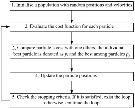
to control the significance of the best solution. The implementation steps of the PSO are illustrated in Figure
7. It is clear that it has a minimum number of parameters that need to be determined. One of the parameters
is population size, which is often set in the range of 20–50, and the values of wand c1, c2 are considered as
unity and two, respectively.
1. Initialise a population with random positions and velocities
2. Evaluate the cost function for each particle
3. Compare particle’s cost with one others, the individual best particle is denoted as pi and the best among particles pg
4. Update the particle positions
5. Check the stopping criteria. If it is satisfied, exist the loop, otherwise, continue the loop
Figure 7: The standard PSO flowchart.
5.2. Regularised PSO
If particle velocities are not restricted when PSO is run, then the velocities can increase to unacceptable levels
within a few iterations. Therefore, this approach was modified by the introduction of constriction coefficients
to regulate particle velocities [44]. The coefficient controls the particle movements and directs them toward the
convergence. The modified velocities of particles can be represented as follows:
vik+1=wkCFv k
i +C1r1(pki −x k
i) +C2r2(pkg−x k
i) (20)
wherewCF =wCF, andC1,C2refer to cognitive and social components that have an influence on convergence
speed and the finding of an optimal point in the search space. The C1 andC2 can be represented as follows:
C1=CF φ1 (21)
C2=CF φ2 (22)
where
CF = 2
|φ−2 +pφ2−4φ|
φ=φ1+φ2
φ1+φ2≥4
where CF and φ represent a constriction factor and co-efficient, respectively. Generally, φ is set 4.1 where
φ1=φ2. Now, the constriction particles can help to converge the process toward optimal solutions without
using velocity limits. However, a better approach is to use limits of velocities and positions.
5.2.1. The procedure for the application of the PSO algorithm
230
The following procedure is applied while evaluating the cost function of each hour.
Part I: Initialisation
0 10 20 30 40 50 60 70 80 90 100
Time (h)
0 5 10 15 20 25 30 35 40 45
Energy (kWh)
10 15 20 25 30 35 40 45
Electricity price (cents/kWh)
Load RE Battery Ct
(a)
10 15 20 25 30 35 40
Electricity price (cents/kWh)
0 10 20 30 40 50 60 70 80 90 100
Time (h)
-20 -10 0 10 20 30
Energy (kWh)
Grid energy Ct
(b)
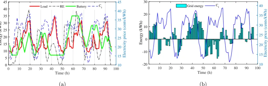
Figure 8: Original cost function for Scenario 1: (a) charging/discharging cycles of the battery energy and (b) energy exchanges
with the grid.
2. Load meteorological data (hourly wind speed, solar irradiation and load profile);
3. Calculate total loads, wind power and solar power;
235
4. Set the parameter of the PSO:
(a) Search space dimension = 1;
(b) Population size = 50;
(c) Maximum number of iteration = 100;
(d) Constriction co-efficient,φ= 4.1;
240
(e) Damping ratio of inertia coefficient,wdamp = 0.99;
(f) Inertia coefficient,w= 0.73;
(g) Penalty factor = 106;
Part II: Iteration for the real-time evaluation
1. For each particle, the position and velocity vectors are randomly selected;
245
2. Evaluate the objective functions to find the fitness value of each particle;
3. Internal iteration start:
(a) Update the velocity and position of each particle according to Eqs. (20) and (19), respectively, while
taking into account their limits;
(b) Calculate the objective function while all constraints are satisfied, otherwise impose penalty factor
250
to discard the solution;
(c) Set the individual best and global best value by comparing the cost function values;
(d) Update inertia weight;
0 10 20 30 40 50 60 70 80 90 100 Time (h) 0 5 10 15 20 25 30 35 40 45 Energy (kWh) 10 15 20 25 30 35 40 45
Electricity price (cents/kWh)
Load RE Battery Ct
(a) 10 15 20 25 30 35 40
Electricity price (cents/kWh)
0 10 20 30 40 50 60 70 80 90 100
Time (h) -20 -10 0 10 20 30 Energy (kWh)
Grid energy Ct
(b)
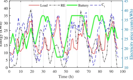
Figure 9: Alternative cost function for Scenario 1: (a) charging/discharging cycles of the battery energy and (b) energy exchange
with the grid.
0 10 20 30 40 50 60 70 80 90 100
Time (h) 0 5 10 15 20 25 30 35 40 45 Energy (kWh) 10 15 20 25 30 35 40 45
Electricity price (cents/kWh)
Load RE Battery Ct
Figure 10: Proposed cost function for Scenario 1: optimal charging/discharging cycles of the battery energy.
6. Simulation results
255
In this section, numerical experiments and comparisons are demonstrated to examine the performance of the
proposed cost function. In this paper, a grid-connected microgrid is considered, where the EMS unit manages
the energy flow of the sources ensuring load demand of the community microgrid in order to reduce operational
costs. The electricity cost is minimised by optimal battery operations as a function of power generation, load
demand and electricity prices, with the application of the regularised PSO algorithm. The battery capacity is
260
chosen as 35 kWh, and the lower and upper storage limits are considered as 7 kWh and 35 kWh, respectively.
The initial energy level of the battery is taken as 17.5 kWh. Table 1 displays the other input values of the
microgrid parameters. Data are taken from real-measurements but they are scaled suitably to apply to this
study. The simulation is calculated over a 96-hour horizon with a time slot of 1 h.
6.1. Scenario 1
265
Case 1: With original cost function
Generally, researchers consider the cost of buying electricity from the grid utility depending on electricity prices
over the time periods [45, 37, 38, 23]. This is formulated asPg×Ct, wherePgis a decision function, consisting
of loads, renewable energy and energy dispatch of the battery. If only this cost function without a square
root is applied to obtain the optimal values for the application of the PSO algorithm, this, indeed, provides
270
only the discharging of the whole battery from the initial energy level, ELo. However, if the cost function is
10 15 20 25 30 35 40
Electricity price (cents/kWh)
0 10 20 30 40 50 60 70 80 90 100
Time (h)
-20 -10 0 10 20 30
Energy (kWh)
Grid energy Ct
(a)
0 10 20 30 40 50 60 70 80 90 100
Time (h)
-4 -2 0 2 4
Battery command, u(t), (kWh)
(b)
Figure 11: Proposed cost function for Scenario 1: (a) energy exchange with the grid and (b) command signals for the battery
energy.
0 10 20 30 40 50 60 70 80 90 100
Time (h)
0 5 10 15 20 25 30 35
Energy (kWh)
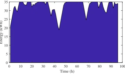
Figure 12: Reserved battery energy for special events.
to only positive values of the function. It is observed that the battery energy is being discharged from the initial
time, t= 0, to feed the loads as RESs are not producing power. The battery is only charged when renewable
power is higher than the load demand, and it is discharged when load demand is higher than the local power
275
supply. The reason for this scenario is that the cost function is developed for discharging the battery power
in order to minimise electricity costs; however, the battery is charged when renewable energy is more than the
load demand due to the square root terms. In this simulation, the total electricity cost for the application of
renewable energy and battery is $38.59 for a time horizon of 96 hours after actively engaging in the electricity
business. It is noticeable from Figures 8a and 8b that the algorithm does not take into account the electricity
280
prices to charge and discharge the battery energy.
Case 2: With alternative cost function
To charge the battery from the RESs and grid utility supply, a charging term that corresponds to the absence of
full charge needs to be added to incur an additional cost in the objective function. This is done mathematically
asBLmax−(BL+u), which always provides an extra cost if the battery is not fully charged. The square root 285
for both terms, charging and discharging, is applied at the function to charge the battery from the RESs and
grid utility [39, 33, 40]. After adding the term to the objective function with a square root, the simulation
results are observed in Figure 9. The battery is charged during low electricity prices up to a certain time,t =
4 h, while power is drawn from the grid utility for loads as well. After that, the battery discharges the power
to feed loads to reduce electricity costs when electricity prices are high. It is also observed that the battery is
290
0 10 20 30 40 50 60 70 80 90 100 Time (h) 0 5 10 15 20 25 30 35 40 45 Energy (kWh)
Proposed Alternative Original Ct
(a)
0 10 20 30 40 50 60 70 80 90 100 Time (h) -20 -10 0 10 20 30 Energy (kWh) 10 15 20 25 30 35 40
Electricity price (cents/kWh)
Proposed Alternative Original Ct
(b)
Figure 13: Comparison for Scenario 1: (a) optimal charging/discharging cycles of the battery energy and (b) energy exchange with
the grid.
0 10 20 30 40 50 60 70 80 90 100
Time (h) 0 5 10 15 20 25 30 35 40 45 Energy (kWh) 10 15 20 25 30 35 40 45
Electricity price (cents/kWh)
Load RE Battery Ct
(a) 10 15 20 25 30 35 40
Electricity price (cents/kWh)
0 10 20 30 40 50 60 70 80 90 100
Time (h) -30 -20 -10 0 10 20 30 Energy (kWh)
Grid energy Ct
(b)
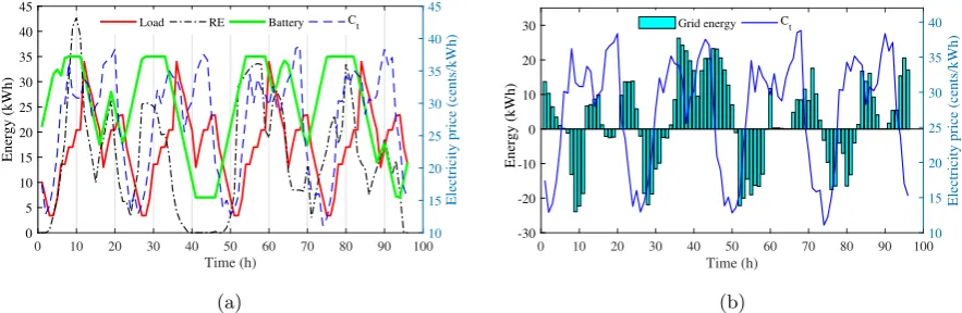
Figure 14: Proposed cost function for Scenario 2: (a) optimal charging/discharging cycles of the battery energy and (b) energy
exchange with the grid.
endeavours to provide an optimal solution based on the defined cost function. However, due to the lack of a
proper formulation, it still struggles to find an optimal solution. The electricity cost of this method is $36.11
for a time horizon of 96 hours.
Case 3: With proposed cost function
295
The limitations of the alternative cost function can be overcome by multiplying a penalty function with the
charging component for not charging the battery during low electricity prices and renewable energy availability.
This penalty function can be static or dynamic based on the electricity prices. However, the static penalty
function generally fails to optimally charge the battery if a varying electricity price is applied because of not
following up its variation. Therefore, this paper proposes a dynamic penalty function that is based on the
300
electricity prices asfpc(C) =k−C(t). The value ofkcan be tuned for receiving the optimal operation of the
battery energy. For example, if owners want to fully charge the battery, the value of kneeds to be increased.
Generally, it is set at the average values of electricity prices, in this paper it is chosen as 29.2. The proposed
penalty function is basically the opposite value of the cost function, which dynamically penalises the objective
function if the battery is not charged optimally from RESs and the grid utility. The result from this cost
305
function is demonstrated in Figures 10 and 11. It is observed that the charging and discharging cycles of the
battery are similar to the alternative function, but with reduced operational costs as $33.76 for a time horizon
of 96 hours. It can be seen from Figure 10 that the storage system discharges its energy to the lowest energy
0 10 20 30 40 50 60 70 80 90 100
Time (h)
0 5 10 15 20 25 30 35 40
Energy (kWh)
Proposed Alternative Original
Figure 15: Comparison among proposed, alternative and original cost functions for Scenario 2.
Table 2: Comparison among cost functions in Scenario 1.
Cost function Electricity cost % Saving
Original (10) 38.57 0
Alternative (11) 36.11 6.38
Proposed (12) 33.76 12.47
power and high cost involvement in charging the battery. Similarly, the battery reaches the highest energy
310
level at time t= 55 h, and the battery is in an inactive mode until t = 66 h due to higher power generation
from RESs. It should be pointed out that the formulation takes into account using the battery energy to send
power to loads when power generation is less than power demand rather than selling power to the grid utility
during high electricity prices. The most important part of this dynamic penalty function is that it can modify
the charging and discharging cycles according to the needs of customers. For example, the battery can be fully
315
charged by adjusting the penalty function prior to any forthcoming events, such as cloudy and rainy days,
where there is a possibility of the loss of electricity connection. Taking into consideration such an event, Figure
12 depicts a full charging battery scenario for a predicted event, where the battery always tries to maintain full
charge, with the expense of electricity cost $38.33, which is still less than the original cost but with maintaining
high energy levels during all the time periods. A comparative study of different functions for energy exchange
320
with the grid utility and optimal battery control is shown in Figure 13 from which it can be seen that the
charging/discharging cycles for the original cost function are different from the proposed and alternative ones.
6.2. Scenario 2
Although the wind speed is the same as in Figure 2, the solar irradiation and daily load patterns are
changed as in Figures 4b and 5b, respectively, to exhibit the effectiveness of the proposed function. The new
325
solar irradiation generates less power than the previous one in Figure 4a. From Figure 14, it is observed that
the battery is charged during low electricity prices and high power generation, and it is discharged during low
power generation and high prices. A comparison of the original, alternative and proposed functions in Scenario
2 is demonstrated in Figure 15 from where the electricity costs are tabulated in Table 3. As can be seen from
Table 3, the electricity cost for the application of the proposed cost function is $60.82 over a time horizon of
330
Table 3: Comparison among cost functions in Scenario 2.
Cost function Electricity cost % Saving
Original (10) 68.68 0
Alternative (11) 62.61 8.84
Proposed (12) 60.82 11.44
the improvement with respect to the alternative cost function is reduced (from 6% to 3% approximately) in
Scenario 2 than that of Scenario 1. This is because of variation in power generation over the peak prices. It
can be concluded that the proposed cost function is superior to the other functions.
7. Conclusion
335
This paper proposes a penalty function multiplied with the charging component of the objective function in
order to obtain optimal use of battery energy by controlling charging/discharging behaviours. In the proposed
function, the constant value can be tuned according to the requirements of the microgrid’s investors. A
meta-heuristic algorithm is applied to facilitate the analysis of the cost functions reported in the literature and the
one proposed here. It is observed that the proposed cost function reduces electricity costs of the community
340
microgrid by around 12% when compared with the original cost function over a time horizon of 96 hours.
Numerical results and comparisons are carried out to demonstrate the effectiveness of the proposed function,
and it can be concluded that the performance of the proposed cost function is superior to other functions.
In future work, the effectiveness of the proposed cost function will be evaluated in an experimental set up,
where the degradation cost of a battery will be taken into account. In addition, a mathematical relationship
345
will be established to accurately determine thekvalue for different energy level stages.
Acknowledgment
This work is supported by the Australian Government Research Training Program (RTP) Scholarship at
The University of New South Wales - Canberra, Australia.
References
350
[1] M. A. Hossain, H. R. Pota, M. J. Hossain, A. M. O. Haruni, Active power management in a low-voltage
islanded microgrid, International Journal of Electrical Power & Energy Systems 98 (2018) 36–47.
[2] A. S. Hassan, L. Cipcigan, N. Jenkins, Optimal battery storage operation for pv systems with tariff
incentives, Applied Energy 203 (2017) 422–441.
[3] M. A. Hossain, H. R. Pota, A. M. O. Haruni, M. J. Hossain, Dc-link voltage regulation of inverters to
355
enhance microgrid stability during network contingencies, Electric Power Systems Research 147 (2017)
[4] R. H. Lasseter, Microgrids, in: Power Engineering Society Winter Meeting, 2002. IEEE, Vol. 1, IEEE,
2002, pp. 305–308.
[5] M. A. Hossain, H. R. Pota, W. Issa, M. J. Hossain, Overview of ac microgrid controls with
inverter-360
interfaced generations, Energies 10 (9) (2017) 1300.
[6] H. Li, A. T. Eseye, J. Zhang, D. Zheng, Optimal energy management for industrial microgrids with
high-penetration renewables, Protection and Control of Modern Power Systems 2 (1) (2017) 12.
[7] M. A. Hossain, H. R. Pota, M. J. Hossain, F. Blaabjerg, Evolution of microgrids with converter-interfaced
generations: Challenges and opportunities (2018), preprints.
365
[8] H. Ibrahim, A. Ilinca, J. Perron, Energy storage systemscharacteristics and comparisons, Renewable and
sustainable energy reviews 12 (5) (2008) 1221–1250.
[9] G. K. Venayagamoorthy, R. K. Sharma, P. K. Gautam, A. Ahmadi, Dynamic energy management system
for a smart microgrid, IEEE transactions on neural networks and learning systems 27 (8) (2016) 1643–1656.
[10] Q. Wei, D. Liu, F. L. Lewis, Y. Liu, J. Zhang, Mixed iterative adaptive dynamic programming for optimal
370
battery energy control in smart residential microgrids, IEEE Transactions on Industrial Electronics 64 (5)
(2017) 4110–4120.
[11] G. P. Henze, R. H. Dodier, Adaptive optimal control of a grid-independent photovoltaic system, in: ASME
Solar 2002: International Solar Energy Conference, American Society of Mechanical Engineers, 2002, pp.
139–148.
375
[12] F. De Angelis, M. Boaro, D. Fuselli, S. Squartini, F. Piazza, Q. Wei, Optimal home energy management
under dynamic electrical and thermal constraints, IEEE Transactions on Industrial Informatics 9 (3) (2013)
1518–1527.
[13] A. C. Luna, N. L. Diaz, F. Andrade, M. Graells, J. M. Guerrero, J. C. Vasquez, Economic power dispatch of
distributed generators in a grid-connected microgrid, in: Power Electronics and ECCE Asia (ICPE-ECCE
380
Asia), 2015 9th International Conference on, IEEE, 2015, pp. 1161–1168.
[14] A. C. L. Hern´andez, N. L. D. Aldana, M. Graells, J. C. V. Quintero, J. M. Guerrero,
Mixed-integer-linear-programming-based energy management system for hybrid pv-wind-battery microgrids: Modeling, design,
and experimental verification, IEEE Transactions on Power Electronics 32 (4) (2017) 2769–2783.
[15] Y. Choi, H. Kim, Optimal scheduling of energy storage system for self-sustainable base station operation
385
considering battery wear-out cost, Energies 9 (6) (2016) 462.
[16] A. Chaouachi, R. M. Kamel, R. Andoulsi, K. Nagasaka, Multiobjective intelligent energy management for
a microgrid, IEEE Transactions on Industrial Electronics 60 (4) (2013) 1688–1699.
[17] Q. Wei, G. Shi, R. Song, Y. Liu, Adaptive dynamic programming-based optimal control scheme for energy
storage systems with solar renewable energy, IEEE Transactions on Industrial Electronics 64 (7) (2017)
390
[18] S. Teleke, M. E. Baran, S. Bhattacharya, A. Q. Huang, Rule-based control of battery energy storage
for dispatching intermittent renewable sources, IEEE Transactions on Sustainable Energy 1 (3) (2010)
117–124.
[19] Y. Riffonneau, S. Bacha, F. Barruel, S. Ploix, Optimal power flow management for grid connected pv
395
systems with batteries, IEEE Transactions on Sustainable Energy 2 (3) (2011) 309–320.
[20] O. Penangsang, A. Soeprijanto, A. A. Fitriana, E. S. Ningrum, Operation optimization stand-alone
micro-grid using firefly algorithm considering lifetime characteristics of battery, in: Intelligent Technology and
Its Applications (ISITIA), 2016 International Seminar on, IEEE, 2016, pp. 565–570.
[21] B. V. Mbuwir, F. Ruelens, F. Spiessens, G. Deconinck, Battery energy management in a microgrid using
400
batch reinforcement learning, Energies 10 (11) (2017) 1846.
[22] T. Huang, D. Liu, Residential energy system control and management using adaptive dynamic
program-ming, in: Neural Networks (IJCNN), The 2011 International Joint Conference on, IEEE, 2011, pp. 119–124.
[23] G. Shi, Q. Wei, D. Liu, Optimization of electricity consumption in office buildings based on adaptive
dynamic programming, Soft Computing 21 (21) (2017) 6369–6379.
405
[24] H. Borhanazad, S. Mekhilef, V. G. Ganapathy, M. Modiri-Delshad, A. Mirtaheri, Optimization of
micro-grid system using mopso, Renewable Energy 71 (2014) 295–306.
[25] C. Justus, Wind energy statistics for large arrays of wind turbines (new england and central us regions),
Solar Energy 20 (5) (1978) 379–386.
[26] S. Rehman, N. M. Al-Abbadi, Wind shear coefficients and energy yield for dhahran, saudi arabia,
Renew-410
able Energy 32 (5) (2007) 738–749.
[27] R. Farrugia, The wind shear exponent in a mediterranean island climate, Renewable Energy 28 (4) (2003)
647–653.
[28] B. S. Borowy, Z. M. Salameh, Optimum photovoltaic array size for a hybrid wind/pv system, IEEE
Transactions on energy conversion 9 (3) (1994) 482–488.
415
[29] W. Xiao, M. G. Lind, W. G. Dunford, A. Capel, Real-time identification of optimal operating points in
photovoltaic power systems, IEEE Transactions on Industrial Electronics 53 (4) (2006) 1017–1026.
[30] A. Kaabeche, M. Belhamel, R. Ibtiouen, Sizing optimization of grid-independent hybrid photovoltaic/wind
power generation system, Energy 36 (2) (2011) 1214–1222.
[31] Overall efficiency of photovoltaic inverters, European Standard EN 50530, 2010.
420
[32] A. C. Nanakos, E. C. Tatakis, N. P. Papanikolaou, A weighted-efficiency-oriented design methodology
of flyback inverter for ac photovoltaic modules, IEEE Transactions on Power Electronics 27 (7) (2012)
[33] D. Fuselli, F. De Angelis, M. Boaro, S. Squartini, Q. Wei, D. Liu, F. Piazza, Action dependent heuristic
dynamic programming for home energy resource scheduling, International Journal of Electrical Power &
425
Energy Systems 48 (2013) 148–160.
[34] A. Bakirtzis, P. Dokopoulos, Short term generation scheduling in a small autonomous system with
uncon-ventional energy sources, IEEE Transactions on power systems 3 (3) (1988) 1230–1236.
[35] D. Liu, Y. Xu, Q. Wei, X. Liu, Residential energy scheduling for variable weather solar energy based on
adaptive dynamic programming, IEEE/CAA Journal of Automatica Sinica 5 (1) (2018) 36–46.
430
[36] ComEd, USA, http://www.thewattspot.com/.
[37] M. Boaro, D. Fuselli, F. De Angelis, D. Liu, Q. Wei, F. Piazza, Adaptive dynamic programming algorithm
for renewable energy scheduling and battery management, Cognitive Computation 5 (2) (2013) 264–277.
[38] G. Shi, Q. Wei, D. Liu, An adaptive dynamic programming based method for optimization of electricity
consumption in office buildings, in: Neural Networks (IJCNN), 2016 International Joint Conference on,
435
IEEE, 2016, pp. 4551–4556.
[39] S. Squartini, M. Boaro, F. De Angelis, D. Fuselli, F. Piazza, Optimization algorithms for home energy
resource scheduling in presence of data uncertainty, in: Intelligent Control and Information Processing
(ICICIP), 2013 Fourth International Conference on, IEEE, 2013, pp. 323–328.
[40] N. Gudi, L. Wang, V. Devabhaktuni, A demand side management based simulation platform incorporating
440
heuristic optimization for management of household appliances, International Journal of Electrical Power
& Energy Systems 43 (1) (2012) 185–193.
[41] H. P. Gavin, J. T. Scruggs, Constrained optimization using lagrange multipliers, CEE 201L. Duke
Univer-sity.
[42] J. Kennedy, R. Eberhart, C. 1995. particle swarm optimization, in: IEEE International Conference on
445
Neural Networks (Perth, Australia), IEEE Service Center, Piscataway, NJ, pp. 1942–1948.
[43] R. Poli, J. Kennedy, T. Blackwell, Particle swarm optimization, Swarm intelligence 1 (1) (2007) 33–57.
[44] M. Clerc, J. Kennedy, The particle swarm-explosion, stability, and convergence in a multidimensional
complex space, IEEE transactions on Evolutionary Computation 6 (1) (2002) 58–73.
[45] T. Huang, D. Liu, A self-learning scheme for residential energy system control and management, Neural
450