Analysis of the cavitating flow induced by an ultrasonic horn

(1)

a

Corresponding author: [email protected]

– Numerical 3D simulation for the analysis of vapour structures and the

assessment of erosion-sensitive areas

Stephan Mottyll1,a, Saskia Müller1, Philipp Niederhofer2, Jeanette Hussong1, Stephan Huth2 and Romuald Skoda1 1

Ruhr-Universität Bochum, Chair of hydraulic fluid machinery, 44801 Bochum, Germany 2

Ruhr-Universität Bochum, Chair of materials technology, 44801 Bochum, Germany

Abstract: This paper reports the outcome of a numerical study of ultrasonic cavitation using a CFD flow algorithm based on a compressible density-based finite volume method with a low-Mach-number consistent flux function and an explicit time integration [15; 18] in combination with an erosion-detecting flow analysis procedure. The model is validated against erosion data of an ultrasonic horn for different gap widths between the horn tip and a counter sample which has been intensively investigated in previous material studies at the Ruhr University Bochum [23] as well as on first optical in-house flow measurement data which is presented in a companion paper [13]. Flow features such as subharmonic cavitation oscillation frequencies as well as constricted vapour cloud structures can also be observed by the vapour regions predicted in our simulation as well as by the detected collapse event field (collapse detector) [12]. With a statistical analysis of transient wall loads we can determine the erosion sensitive areas qualitatively. Our simulation method can reproduce the influence of the gap width on vapour structure and on location of cavitation erosion.

Nomenclature

= Density []

c_s = Speed of sound [ ]

= Vapour volume fraction []

x = Vapour mass fraction []

s0 = Constant entropy [ ]

u = Velocity vector [ ]

=

Relative massflow at cell-face

[ ]

p = Pressure [Pa]

= Erosion probability by

pressure indicator

[]

condensation rate indicator

[]

combined erosion indicator

[]

=

Scaled pressure []

=

Volume of computational cell []

!"

=

Reference length []

=

Collapse pressure []

f_rel,std =

Relative standard-deviation [] f_rel,_#$ =

Relative maximal-deviation []

f_sub =

Subharmonic frequency [Hz]

Tsub =

Subharmonic time period []

f_%!&' =

Driving frequency [Hz]

()

=

Peak-to-peak amplitude [µ m]

*+ *+ *, =

Analysis time-intervals

[s]

Subscripts

baro = Barotropic value

v = Vapour phase

L = Left state

R = Right state

face = State at cell face

init

= Initial condition

grd = State: moving grid

1 Introduction

Despite the importance of cavitating flows in hydraulic fluid machinery, there are no CFD methods for the reliable prediction of cavitation erosion (incubation time, erosion rate, location of erosion) available.

The overall objective of our research is the numerical modelling of cavitation to predict erosive damage on material surfaces.

C

(2)

As a function of intensity and frequentness, near-wall collapses of vapour bubbles/clouds in cavitating flows lead to material fatigue and erosive damage. Theoretical investigations predict that wall-near or wall-bounded single bubbles emit shock waves with maximal pressures far above 1000 bar [1]. These shock waves are transported with speed of sound, requiring a very high temporal resolution. Due to the complexity of this phenomenon the simulation of cavitating flows and resulting cavitation erosion is still a challenging task.

There exist different methods for the simulation of cavitating flows: Interface tracking methods, volume of fluid (VoF) methods, discrete bubble methods, two-phase flow methods (component methods or multiple species methods) [8; 20]. Although these methods are widely used, most of them are not suitable to predict the driving mechanisms of cavitation erosion. They cannot determine wave propagation at speed of sound since they are based on incompressible, pressure based flow algorithms and on implicit time integration schemes.

An alternative to these numerical methods is to capture details of the compressible wave dynamics of cavitating flows by using a density-based method with a high temporal resolution. In this paper we analyse a modelling approach based on a compressible density- based finite volume method with a low-Mach-number consistent flux function and an explicit time integration [15; 18]. Phase change between vapour and fluid is taken into account by a barotropic equation of state assuming thermodynamic equilibrium and a homogeneous mixture in each cell.

In the past, cavitation erosion has been analysed with this density-based flow algorithm and barotropic cavitation model for case of hydrodynamic cavitation, e.g. for hydrofoils [21], axisymmetric nozzles [11; 12] or micro channels [12; 22]. Simulation results show a good agreement with measurement data for the location of cavitation erosion damage. Dular et al. [4] and Mettin et al. [9] have analysed ultrasonic cavitation at an ultrasonic horn tip by using of different VoF-Models (Schnerr-Sauer [14], Zwart-Gerber-Belamri [26], Singhal [19]). In spite of systematic parameter variation for cavitation model parameters they cannot capture the subharmonic cavitation oscillation frequencies. Cavitation expansion is calculated immensely faster and the maximum amount of vapour achieved is much lower than in experimental measurements. They concluded that these cavitation models are not appropriate for the simulation of ultrasonic cavitation and further modifications of present cavitation models are needed [4].

In our research we will apply the density-based flow algorithm with barotropic cavitation model to describe ultrasonic cavitation. The model will be validated on a testcase of an ultrasonic horn which is well examined in previous research at the Ruhr University Bochum [11]. To evaluate the erosion sensitive areas we use a statistical analysis of transient wall loads [21; 22]. We trace the location of isolated collapse events with an analysis method referred to as collapse detector [10; 11; 12; 16]. Based on the field of detected collapse events we estimate the vapour cloud structure.

In a first validation step we compare the determined erosion sensitive areas to the experimental data for the location of erosive damage (surface contours) at ultrasonic horn samples for different gap widths. In a second step, we analyse the vapour cloud structures for different gap widths. We compare the field of collapse events as well as the vapour regions (iso-surfaces) predicted in our simulation to shadowgraph images of the bubble field. In a companion paper measurement data for the same flow geometry are shown [13].

2 Physical model

Because the driving effects behind cavitation erosion are inertia driven (compressible wave propagation) [5; 17], we assume that viscous effects are negligible and apply the compressible Euler equation for mass and momentum conservation. We adopt a homogeneous mixture of liquid and vapour assuming both phases to be present at thermodynamic equilibrium, which also means that phase transition (vapourisation and condensation) occurs instantaneously. As a result, energy equation can be neglected and phase change follows an isentropic path. The influence of air, neither undissolved nor dissolved, will not be taken into account. Hence, the density of the fluid is only dependent on pressure, which is commonly referred to as barotropic model [7].

To take the coupling between density and pressure into account we use an equation of state based on the reference equations by the industrial standard formulation IAPWS-IF97 for water [25]. We apply lookup-tables for barotropic density, speed of sound, vapour mass fraction and vapour volume fraction as a function of mixture pressure and constant entropy (isentropic path at thermodynamic equilibrium):

_baro, cs+baro, v, xv=f(p,s0)

(1)

3 Underlying numerical method

We employ our flow simulation code hydRUB (hydraulic Ruhr University Bochum), with a numerical method developed at the Munich University of Technology [15; 18] which is summarised here for the sake of completeness.

The numerical scheme has a Low-Mach number consistent Gudonov-type flux formulation. By defining the state at the cell faces using the following equation

uface= 1

L+R-LuL

+_RuR+pL-pR

cs,face. (2) p_face=1/₂0p_L+p_R1 (3)

cs, face=max0cs,L,cs,R1, (4) Euler fluxes can be defined as

F=ȡ_L/RÂu_faceÂ 2222 1 u3_////₄

v3_////₄

w3_////₄

5 5 5 5 + 6666

0 p_face

0 0

7 7 7

(3)

The left (L) and right (R) states are calculated in upwind direction dependent on the sign of uface. By using this flux formulation for the description of convective fluxes in our governing equations it is possible to describe pressure wave propagation in liquids. To resolve pressure waves at speed of sound, the numerical time step has to be necessarily proportional to the ratio of the minimum grid size and the fastest signal speed (maximum speed of sound plus liquid velocity). As a consequence, we employ a 4th order explicit Runge-Kutta time integration scheme with a fixed CFL-number smaller than one (stability region). The spatial reconstruction of velocity field and density has been applied by the monotonic TVD (Total Variation Diminishing) limiter “minmod” [6]. Hence, the resulting numerical approach is 2nd order accurate in space and time [6].

For the simulation of ultrasonic horn tip oscillation we extend the method by a numerical algorithm to describe grid movement. In order to ensure that no artificial mass sources/sinks are induced by the grid movement, we use the space conservation law (SCL) to determine grid mass flow [2; 3]. The convective fluxes at the cell-faces are determined with a relative mass flow rate mre which is defined as the difference between fluid mass flow rate and grid induced mass flow rate. If the grid induced mass flow rate is calculated by the change of the cell volume it automatically satisfies the SCL [2]. In order to reduce numerical inaccuracy we solve the SCL with the same time integration scheme as the governing equations.

The grid kinematic has been updated every Runge-Kutta time-step to ensure that no mass defect takes place during the inner Runge-Kutta Loops. The implementation of oscillating grid kinematics in combination with space conservation has been validated at different basic testcases (Lid Driven Cavity, Piston Movement). Thereby it could be ensured that no artificial mass source or sink occurs.

We apply body-fitted, block structured hexahedral grids for the discretisation of flow field. The block structure is chosen in a way, that almost linear scaling on multi-processor system is possible.

3.1 Analysis methods

For the analysis of location of erosion sensitive areas and vapour cloud structures we use two different numerical approaches: a statistical analysis of the transient wall load and the so called collapse detectors.

3.1.1 Statistical analysis of transient wall loads

For the statistical analysis of wall loads, we assume that the erosion probability can be estimated by two indicators: pressure and negative gradient of vapour volume fraction (condensation rate).

In a first step we cut-off the pressure and condensation rate at a fixed location to tell apart the bulk value from the peaks value. We assume that these indicator peaks determine the wall stress. For the cut-off

a series of threshold values is utilized for both indicators. As a function of the wall coordinates we determining the ratio of the indicator peaks exceeding the threshold and the number of prescribed analyse time-steps. In this way, we obtain a pressure probability Pp and a condensation probability P, for a predefined time interval [22].

As it could be worked out in previous research [21], the combination of these single erosion indicators leads to a probability Pcomb = PP P which specifies erosion

sensitive areas.

3.1.2 Collapse Detector

In order to detect and evaluate single collapse events within the flow field we use a numerical approach further referred to as ‘Collapse Detector’ [12].

The main idea of the Collapse Detector is to define a set of physical criteria to detect collapses of isolated vapour clouds and to characterise the strength of resulting shock waves. Figure 1 shows a schematic sketch of the consecutive stages of a vapour cloud collapse. At the beginning of collapse, the vapour cloud starts to condense; hence, the velocity field is directed towards the centre of the cloud corresponding to a negative divergence of the velocity field. The surrounding liquid is further accelerated towards the centre until the vapour completely condenses directly at the stage of collapse. At this instance in time, the pressure rises intensely developing a shock wave and leading to an outward directed velocity field (divergence of the velocity field changes its direction) [12].

Figure 1. Sketch of consecutive stages of vapour structure collapse over the divergence of velocity field [12].

As vapour volume vanishes and a change in the direction of the velocity field takes place, the actual time-step as well as the position, the maximum pressure and the condensation rate of the affected cells are stored for post-processing.

In order to reduce the effect of remaining grid inhomogeneity for the determined collapse pressure, we apply a linear decay law and scale the collapse pressure to a uniform length scale, x_re₈ [11].

p_scale~9Vcell 3

xref pcollapse

(4)

collapse detector only as an indicator for the local vapour cloud structure and to get a qualitative overview of the position of violent collapses.

4 Testcase

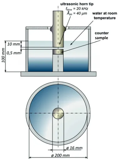
As simulation testcase we choose an ultrasound horn setup further referred to as sonotrode [23]. In this setup, a sonotrode horn tip oscillates with a frequency of 20 kHz and peak-to-peak amplitude of 40 µm above a counter sample inducing a cavitating flow (cf. Fig. 1). The gap width between sonotrode horn and counter sample amounts to 0.5 mm which is optimised for cavitation erosion analysis at counter sample surface for stainless steel (1.4462) [23].

The sonotrode tip oscillates inside a cubic reservoir filled with non-degased distilled water at room temperature. First experiments show circular vapour structures growing and collapsing periodically inside the gap. Due to vapour structure collapses inside the gap, material is eroded at the horn surfaces and the counter sample surface, after a short incubation phase. The resulting surface contour at the counter sample strongly depends on the operation point of the oscillation movement (frequency, amplitude, gap width) [23].

Figure 2. Schematically sketch of the simulated ultrasonic horn geometry.

5 Numerical setup

We choose a rotationally symmetric segment geometry with a rotation angle of 90° as computational domain in order to reduce the numerical effort (cf. Figure 2), although we are aware of the fact that cavitation is always three-dimensional and non-periodic. As a result, the side planes are implemented as periodic interfaces. All solid boundaries are chosen to be slip-walls, as we neglect the viscous effects. For the 90°-segment we simulate the flow

domain up to the reservoir walls to account for pressure wave reflections which we assume to have an important influence on the flow field. The horn tip surface is implemented with oscillating grid kinematic of 40 µm peak-to-peak amplitude and a frequency of 20 kHz.

Figure 3. Sketch of the computational domain with all boundary conditions (90° rotation symmetrical segment geometry)

As initial condition we set the velocities inside the complete domain to X and the pressure level to the barometrical pressure . The applied barotropic table is defined for water at the temperature of .

We set up a double O-grid grid topology to adequately reproduce the axial symmetric geometry (cf. Figure 3). The Cell volume is chosen to be nearly constant within the entire gap to reduce grid dependency for erosion analyse. As additional consequence in combination with the CFL-condition (CFL = 0.7), an almost constant local time-step is obtained for every cell inside the gap.

Figure 4. (l) top view of the block topology; (r) hexahedral grid inside the gap.

To estimate grid dependency of our numerical solution we perform a grid sensitivity study. We utilize three grids with increasing spatial resolution, further referred as “coarse” (0.65 mil cells, 19 blocks), “middle” (1.33 mil cells, 38 blocks) and “fine” (2.48 mil cells, 38 blocks). Grids are successively refined within the gap between horn tip and counter sample. Every grid results from the next coarser one by refining each block-discretisation by a factor of approximately 1.2. For one refinement step, the total number of cells is increased by a factor of 2. The resulting numerical time-steps are shown in table 1:

(5)

Table 1. Parameters of the calculations.

coarse middle fine

Numerical

time-step dt :;<= > ?@A B;?: > ?@A ?;=C > ?@A

Simulated physical

time ?;BD ?;:?

?;B:

Number of simulated

time-steps B@@@@@ :<@@@@ C<@@@@

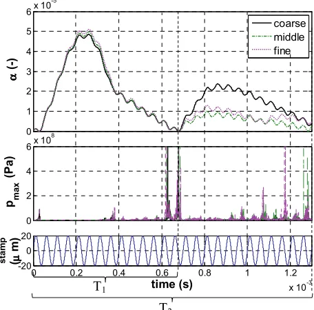
As indicator for grid sensitivity study, we choose the spacial integral vapour volume fraction over the whole computational domain, as it is a decent indicator for the accuracy of our cavitating flow simulation and accordingly also for the cavitation erosion analysis. We analyse the relative standard-deviation related to the maximal value of over time further defined as

f_rel,std = std(grd)

max () (6) and the maximal deviation

f_rel,max = max(grd)

max () (7) where std(grd) is the standard deviation and max(_grd) the maximal deviation of compared to the next coarser grid resolution. As analysis time interval we choose 0 – 1.2 ms (cf. Figure 5).

Figure 5. Integral vapour volume fraction for the grid resolutions: coarse, middle, fine.

For the first subharmonic oscillation time (T1) the difference between all spatial resolutions is relatively small in the range of E!+F% G ?H(cf. Table 2). After T1 we observe that the spatial resolution has a strong influence on the vapour production and collapse dynamics. On the coarse grid the production of vapour is

nearly twice as big as on middle or fine grid. The maximal deviation E!+Ibetween coarse and middle grid resolution is in the range of 27.84 %, between middle and fine grid at 6.07 % (cf. Table 2). However, the standard deviation E!+F%between middle and fine is only 1.97 %.

Table 2. Results of grid sensitivity study.

T1[0 – 0.7] ms T2[0 – 1.2] ms

middle vs. coarse

f_rel_+#$ _{3.05 %} _{27.84 %} f_rel,std _{0.92 %} _{10.47 %}

fine vs. middle

f_rel_+#$ _{3.01 %} _{6.07 %}

f_rel,std _{0.95 %} _{1.97 %}

We assume that a standard deviation lower than 2% is tolerable, so that the middle grid resolution is an appropriate compromise between simulation accuracy and computational effort. All subsequent results are therefore obtained on the middle grid resolution. For higher gap widths the grid was extruded with constant grid resolution.

6 Experimental validation data

6.1 Subharmonic oscillations

Dular et al. [4] and Mettin et al. [9] have shown in their experimental analysis that expansion and collapse of vapour structures take place on subharmonic time scales with respect to the driving frequency [4]. For testcases without counter sample the subharmonic emission falls into the range of 1/7 to 1/5 of the driving frequency [24]. During a subharmonic oscillation cycle the form of vapour clouds changes from “mushroom” to “cone” before collapse. For testcases with counter sample there was no experimental data available.

6.2 Bubble field

In our companion paper [13] the bubble field for different gap widths has been analysed. In shadowgraph images we observe that for moderate gap widths between 1mm and 5mm the bubble field forms a constricted shape. Most of the bubbles can be detected directly at the horn surface or at the counter sample surface (cf. Figure 6). For higher gap widths the shape changes to a cone.

Figure 6. Snapshot from shadowgraph images of the bubble field for different gap widths and actuation amplitudes. a) Gap = 3 mm; JKLLM NOPQ; b) Gap = 5 mm; JKLLM ORPQS?:T.

0 1 2 3 4 5 6x 10

-5

αααα

(-)

0 2 4 6x 10

8

p ma

x

(P

a

)

0 0.2 0.4 0.6 0.8 1 1.2

x 10-3 -20

0 20

time (s)

z stam

p

(μμμμ

m)

coarse middle fine

T1

T2

M BU() M B<P

M <U()M <@P

a)

(6)

6.3 Location of erosion damage

The location of maximal erosive damage at the counter sample surface for different gap widths has been analysed with experimental long-term runs at the Ruhr-Universität Bochum by Stella [23]. He concludes that for higher gap widths the erosive material damage of the counter sample gets lower and the radius of eroded area diminishes (cf. Figure 7).

Figure 7. Eroded surface of a counter sample of copper for different gap widths (0.5 mm; 2.5 mm; 4.5 mm) a

7 Results and discussion

In our numerical investigations, we vary the gap width between sonotrode horn tip and counter sample in order to validate our CFD method on the experimental observations:

1. Expansion and collapse of vapour structures take place on subharmonic time scales (subharmonic cavitation oscillation frequencies).

2. Constricted vapour cloud structures for moderate gap widths.

3. Radius and intensity of eroded surface area diminishes due to increasing gap size.

7.1 Integral vapour volume fraction

Figure 8 shows the time history for T = [0 - 2] ms of the integral vapour volume fraction and integral maximal pressure pmax over the horn tip movement zstamp

a

Measurements and images by Philipp Niederhofer, Chair of materials technology at Ruhr-Universität Bochum.

The driving frequency of the sonotrode horn tip is fdrive = 20 kHz. Subharmonic frequencies ?/*_V for the vapour expansion and collapse can be observed for all three gap widths. Thereby subharmonic emissions fall into the range between 1/9 and 1/13 of the driving frequency (cf. Table 3). For higher gap widths the subharmonic frequency increases.

Table 3. Period time Tsub and frequency fsub for the overlaid sub-harmonic oscillation

Gap width 0.5mm 2.5mm 4.5mm

Period time Tsub @;C< @;< @;:C

Subharm. freq. fsub ?<:@WX Y@@@WX Y?Z@WX

Ratio: fsub/fdrive ?[?B ?[?@ ?[=

Our first impression is that the subharmonic frequencies correlate directly with the strength of the pressure peaks. Collective vapour cloud collapses lead to pressure peaks which follow the same subharmonic frequency. The amount of vapour inside the respective cloud seems to correspond to the strength of the preceding pressure peak. The higher the pressure peak (e.g. Fig. 8, marked with an arrow 1011Pa), the more vapour will be produced in the next vapour cloud. To verify this statement we intend to analyse this phenomenon in further simulations and experiments in future.

7.2 Local vapour cloud structure

On the left side of figure 9 a snapshot of the vapour regions predicted by our simulation tool is shown for different gap widths. View is directed to a periodic interface of the rotational symmetric segment geometry from inside of the domain. Vapour regions are represented by iso-surfaces of vapour volume fraction of = 0.1. In order to get an impression of the general vapour cloud structure, we choose a time instant where vapour volume fraction is nearly maximal.

On the right side of figure 9 the single-collapse events detected inside the gap are shown. Collapses are displayed as spheres and plotted at the position of their occurrence. The colour and diameter of each sphere is scaled with the collapse pressure serving as indicator for collapse intensity.

The local vapour cloud structure is estimated by the iso-surface of vapour volume fraction of = 0.1 and marked with a red shape (cf. Figure 9). Furthermore we mirror the shape to the field of detected collapses (right side of Figure 9). We conclude that the iso-surfaces of the vapour volume fraction correlates directly to the detected collapse field and thus both can be used as indicators for vapour cloud structure.

For a gap size of 0.5 mm the whole gap is nearly filled with vapour. The constriction of the vapour structure is hardly discernible. At 2.5 mm gap size, a full constricted vapour cloud structure can be observed. For a 4.5mm-gap the cloud structure changes towards a constricted cone shape.

0 2 4 6x 10

-5

αααα

(-)

0 5 10x 10

8

p ma

x

(Pa

)

0 0.5 1 1.5 2

x 10-3 -20

0 20

time (s)

z st

am

p

(μμμμ

m)

0,5 mm gap 2,5 mm gap 4,5 mm gap

*V+\;] *V+,;] *V+^;]

(7)

Compared to the enclosing shape of the bubble fields recorded in our shadowgraph images (cf. Figure 6) the determined shapes (cf. Figure 9) looks quite similar [13]. The constricted shape of the bubble field can also be covered by our simulation results for the local vapour cloud structure (collapse detector and iso-surface). In addition, most of the vapour volume can be detected – both in the simulation and in the experiments – directly at the horn surface and at the counter sample surface.

On the right side of Figure 9 we could further observe that most of the violent collapses are detected near the centre line of our computational domain. We estimate that this effect can be ascribed to our rotational symmetric geometry as incoming shock waves can escalate directly at the rotation axis inside the gap where two periodic interfaces are in immediate neighbourhood. Further investigations will be done on full 360°-geometry in the future.

7.3 Erosion probability

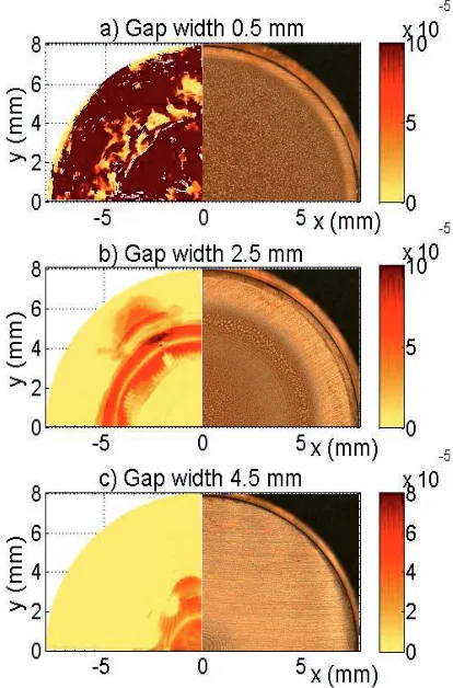
The calculated erosion probabilities at the counter sample surface are documented in Figure 10.

We apply the combined erosion indicator by overlaying pressure and condensation rate indicators for the thresholds: thrp = 7.5e6 Pa and thr = -3e5 s-1.

Colourbar scaling and thresholds are the same for all three gap widths. For the contour plot, dark red coloured sections define regions with high erosion probability and light yellow ones with low erosion probability. The images on the right side of Figure 10 represent the eroded surfaces contour observed in our experiments (cf. Figure 7). The calculated erosion probability allows a qualitatively correct ranging-in of erosion sensitive areas for different gap widths. The erosion probability for the smallest gap size is largest and gets lower with increasing

gap size. Furthermore, the eroded area gets smaller with increasing gap size.

Figure 10. (left) Erosion probability Pcomb as a combination of pressure erosion probability Pp for a threshold of 7.5e6 Pa and condensation erosion probability P_Į for a threshold of -3e5 s-1. (right) Images of experimentally observed erosion damage (cf. measurements of Stella) [23]. a) gap width 0.5 mm; b) gap width 2.5 mm; c) gap width 4.5 mm.

Figure 9. (l) Random single time instant showing iso-surfaces of vapour volume fraction (Į = 0.1) for three different gap widths. The areas marked in red show the potential vapour cloud spectrum which can be observed in experiments to form a constricted shape [1] (r) Visualisation of collapses detected during the analysis interval. Collapses are visualised as spheres at the position of its occurrence.

Colour and size represent the collapse pressure scaled to a uniform reference length __`ab. 0.5 mm

2.5 mm

(8)

We conclude that this circumstance correlates to the change in vapour cloud structure. Modifying the gap width leads to a change in cavitating flow field (cf. Chapter 7.2) and hence to a change in location of eroded surface. For increased gap sizes, vapour cloud structure changes more and more to a cone form with the result that collapses take place more frequently at the centre line of the counter sample surface (cf. Figure 6 and 10). This behaviour could also be observed in the experimental analysis represented in the companion paper. For a greater gap width of 17 mm the vapour cloud structure forms a nearly perfect cone. Shadowgraph images of the measurement results are shown in our companion paper [13].

For 2.5 mm gap size we observe that nearly no erosion probability is predicted in the middle of the counter sample. Since this behaviour is not obvious in the experiment (cf. Figure 7), we intend to compare these results to more detailed measurements of the depth of eroded surface profile in the future.

8 Conclusion and outlook

We have applied our density-based in-house flow solver hydRUB for the simulation of ultrasonic cavitation induced by sonotrode horn tip for different gap widths between sonotrode horn and counter sample. We could range in different gap-variants qualitatively for their erosion sensitive areas, although we neglect viscose effects and energy equation and use a homogeneous mixture approach.

With our numerical model we could observe that expansion and collapse of vapour structures take place on subharmonic time scales (frequencies in the range of 1/9 to 1/13 of the driving frequency). Furthermore we could capture the general behaviour of the experimentally observed bubble field forming a constricted vapour cloud structure insight the gap. The local vapour cloud structure predicted by the collapse field as well as by the iso-surfaces of the vapour volume fraction determines a quite similar shape compared to shadowgraph images presented in our companion paper [13].

We could also evaluate the location of cavitation erosion qualitatively for different gap widths. We observe that increasing the gap size diminishes the erosive damage at the counter sample and reduces the eroded surface area. We conclude that the statistical analysis of transient wall load applied in the present study represents an appropriate method to predict erosion sensitive regions.

Further investigations will be done in order to make a foundation for our present results. We will enhance the simulation time interval to ensure that a steady-state solution has been reached after 3 - 4 subharmonic cavitation oscillation cycles in order to increase the statistical significance. Furthermore we will analyse the influence of the present 90°-segment geometry by comparing the results to those of a full 360° geometry. We will apply additional sensitivity studies for different oscillation amplitudes and reservoir geometries. In future experiments, via confocal light microscopy using a

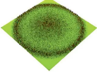
device made by Nanosurf we want to record 3D-surface profiles of the eroded counter sample surfaces for different operation points. A preliminary result is shown in (cf. Figure 11).

Figure 11. 3D-surface profile recorded by a confocal light microscope of the counter sample surface for a gap width of 2.5 mm, a peak-to-peak amplitude of 50 µ m and a driving frequency of 20 kHz.b

Additionally in future studies numerical results of the vapour cloud structure will be validated against shadowgraph images underneath the horn tip showing the radial propagation of the bubble field.

References

[1] C. E. Brennen, Fundamentals of multiphase flow. Cambridge Univ. Press (2006).

[2] I. Demirdžiü, M. Periü. Int. J. Numer. Meth. Fl. 8 9, S. 1037–1050 (1988).

[3] I. Demirdžiü, M. Periü. Int. J. Numer. Meth. Fl. 10 7, S. 771–790 (1990).

[4] M. Dular, R. Mettin, A. Žnidarþiþ, V. A. Truong. 8th Int. Symp. on Cavitation (CAV), Singapore (2012). [5] J.-P. Franc, J.-M. Michel, Fundamentals of

Cavitation. Springer Science + Business Media Inc (Fluid Mechanics and Its Applications, 76) (2005). [6] A. Harten. J. Comput. Phys. 49 3, S. 357–393

(1983).

[7] U. Iben. Sys. Anal. Mod. Sim. 42 9, S. 1283–1308 (2002).

[8] A. H. Koop, Numerical Simulation of Unsteady Three-Dimensional Sheet Cavitation, Dissertation, University of Twente, Enschede (2008).

[9] R. Mettin, M. Dular, A. Žnidarþiþ, V. A. Truong. 38. Jahrestagung für Akustik (DAGA), Darmstadt (2012).

[10] M. S. Mihatsch, S. J. Schmidt, M. Thalhamer, N. A. Adams. 4th Int. Conf. Comp. Meth. Marine Eng. (MARINE), Lisbon (2011).

[11] M. S. Mihatsch, S. J. Schmidt, M. Thalhamer, N. A. Adams. 8th Int. Symp. on Cavitation (CAV), Singapore (2012).

[12] M. S. Mihatsch, S. J. Schmidt, M. Thalhamer, N. A. Adams, R. Skoda, U. Iben. 3rd Int. Cavitation Forum (WIMRC), Warwick (2011).

b

(9)

[13] S. Müller, M. Fischper, S. Mottyll, R. Skoda, J. Hussong. Exp. Fluid Mech. (EFM), Kutná Hora (to be published).

[14] J. Sauer, G. Schnerr. J. Appl. Math. Mech. (ZAMM) 81 (2001).

[15] S. Schmidt, I. Sezal, G. Schnerr, M. Talhamer. 46th Aerosp. Sci. Meeting (AIAA), Reno (2008). [16] S. J. Schmidt, M. S. Mihatsch, M. Thalhamer, N. A.

Adams. 3rd Int. Cavitation Forum (WIMRC), Warwick (2011).

[17] S. J. Schmidt, I. Sezal, G. Schnerr, M. Thalhamer. 8th Int. Symp. Exp. Comp. Aerothermodynamics of Internal Flows (ISAIF), Lyon (2007).

[18] G. H. Schnerr, I. H. Sezal, S. J. Schmidt. Phys. of Fluids 20 4 (2008).

[19] A. Singhal, L. Huiying, A. Jiang. J. Fluids Eng. 124 (2002).

[20] K. T. Sipilä, RANS Analyses of Cavitating Propeller Flows. VTT Technical Research Centre of Finland (VTT science) (2012).

[21] R. Skoda, U. Iben, M. Güntner, R. Schilling. 8th Int. Symp. on Cavitation (CAV), Singapore (2012). [22] R. Skoda, U. Iben, A. Morozov, M. Mihatsch, S.

Schmidt, N. Adams. 3rd Int. Cavitation Forum (WIMRC), Warwick (2011).

[23] J. Stella, Metallkundliche Vorgänge in der Inkubationsphase der Kavitationserosion, Dissertation, Ruhr-Universität Bochum, Bochum (2004).

[24] V. A. Truong. J. Sci. Technol. 73B (2009).

[25] W. Wagner, H.-J. Kretzschmar, International steam tables.2nd ed. Springer (2008).