Stability and Boundedness Properties of a Rational Exponential Difference Equation
J.Leo Amalraj1, M.Maria Susai Manuel2, Adem Kılı¸cman3 and D.S.Dilip4
1Department of Mathematics, RMK College of Engineering and Technology,
Thiruvallur District, Tamil Nadu, India. email: [email protected]
2Department of Mathematics, RMD Engineering College, Thiruvallur District,
Tamil Nadu, India. email: [email protected]
3Department of Mathematics and Institute for Mathematical Research,
University Putra Malaysia, 43400 UPM, Serdang, Selangor, Malaysia
email: [email protected]
4Department of Mathematics, St.John’s College, Anchal, Kerala, India.
email: [email protected]
Abstract
This article aims to discuss, the stability and boundedness character of the
solutions of the rational equation of the form
yt+1 =
ν−yt +δ−yt−1
µ+νyt+δyt−1
, t∈N(0). (1)
Here, >1, ν, δ, µ ∈(0,∞) and y0, y1 are taken as arbitrary non-negative reals and N(a) = {a, a+ 1, a+ 2,· · · }. Relevant examples are provided to validate our results.
The exactness is tested using MATLAB.
Key words: Boundedness, Equilibrium, Global asymptotic stability, Rational Equa-tion.
AMS Classification 2000: 39A22.
1
Introduction
Difference equations involving geometrical and exponential functions have many
applications in biology. Growth of a perennial grass, generally rely on the parameters
biomass, like litter mass and soil nitrogen, was described by the difference equations
Bt+1 =µN
eν−δLt
1 +eν−δLt, Lt+1 = L2
t
Lt+d
+µsN e
ν−δLt
1 +eν−δLt, s∈(0,1). (2)
Here, the parametersB,L and N denote biomass, litter mass, soil nitrogen
respec-tively, ν, δ, µ, d >0 are fixed. Oscillatory behaviour and chaotic climate of (2) was
discussed in [22].
The boundedness, stability and periodic character of the solution obtained
from exponential rational equation
yt+1 =α+βyt−1e−yt, t ∈N(0)
was obtained by El-Metwally et all [13]. The population growth rate β and
immi-gration rateα are positive reals with initial conditions y0 and y1.
Global asymptotic behavior and Boundedness behavior of the difference
equa-tions
yt+1=
α+βe−yt γ+yt−1
,
and
yt+1 =
αe−(tyt+(t−s)yt−s) β+yt+ (t−s)yt−s
, t ∈N(0)
have been developed by Ozturk et all [19, 20], where α > 0, β > 0 and s ∈ N(1)
and they−j for j = 0,1,2,· · · , s can be taken as reals.
For given realsδ, µ, d, sand 0< a <1, the entity of periodical solution is given
by the equation
yt+1 = νy2
t
yt+δ
+µ e
s−dyt
1 +es−dyt.
Authors in [3] discussed stability behaviour of the equation
yt+1 =
αe−yt +βe−yt−1
γ+αyt+βyt−1
, t∈N(0). (3)
Here, the initial conditions are taken as arbitrary reals and α, β are positive
num-bers.
which preserve symmetries. The role of difference equations are well established
in the study of Lie theory. One can refer[10]-[12] for a detailed study on this aspect.
Qualitative properties of certain class of rational difference equations was
ana-lyzed in [8, 4]. Stability and bounded conditions of the equationyt+1 =f(yt)g(yt−s) was developed in [9] and the qualitative behavior ofyt=
f(yt−1, . . . , yt−s)
g(yt−1, . . . , yt−s)
, t∈N(0)
was studied in [2]. For a detailed study on the theory and applications of the
rele-vant topic, one can refer [1], [5]-[7], [14]-[18], [21].
In this paper, we extend the theory to (3) and establish new conditions for
stability and other behaviors of the equations (1) for > 1. MATLAB is used to
test the exactness of the behavior of the solutions.
2
Preliminaries
Definition 2.1. [8] Let f : I × I → I, I ∈ R, be a continuous function and
y0, y−1 ∈I be given values. Then, for
yt+1 =g(yt, yt−1), t ∈N(1) (4)
¯
y is called equilibrium of (4) if f(¯y,y¯) = ¯y.
Definition 2.2. [8] Letp= ∂g
∂u(¯y,y¯) and q= ∂g
∂v(¯y,y¯)denote the partial derivatives
of f(u, v) evaluated at an equilibrium y¯of (1). Then the equation
yt+1 =pyt+qyt−1, t ∈N(0) (5)
is called the linearized equation associated with (1) about the equilibrium point y¯.
The auxillary equation of (5) is the equation
2−p−q= 0 (6)
with characteristic roots± = p±
p
p2 + 4q
2 .
(i) If two roots of (6) are in the region ||<1, then we have an equilibrium y¯of
(1) which is asymptotically and locally stable.
(ii) If at least one of the roots of (6) is in the region||<1, then the equilibrium
¯
y of (1) is unstable.
(iii) The two roots of (6) will lie in the open region ||<1 if and only if
|p|<1−q <2. (7)
This locally asymptotically stable equilibrium point y¯is called a sink.
(iv) The magnitude of one of the two roots of (6) is more than unity if and only if
|1−q|>|p| and |q|>1. (8)
This equilibrium point y¯is called a repeller.
(v) The absolute value of one of the roots of (6) is more than unity and the other
has absolute value less than unity if and only if
|p|>|1−q| and p2+ 4q >0. (9)
and this unstable equilibrium point y¯is called a saddle point.
(vi) If a root of (6) has absolute value unity, then |p| = |1−q| or q = −1 and
|p| ≤2. Conversely, if |p|=|1−q|or q=−1and |p| ≤2 then we get one root
whose absolute value is equal to unity and hence we get the equilibrium point
¯
y, which is non hyperbolic.
3
Main Results
Here, we discuss the existence, uniqueness and stability of the equation (1).
Proof. Let F(y) = (ν+δ)
−y
µ+ (ν+δ)y −y and F(0) = ν+δ
µ >0.
Then, from our assumption, lim
y→∞F(y) =−∞.
This gives us that (1) has equilibrium ¯y.
F0(y) =−
(ν+δ)−yµln+ (ν+δ)(yln+ 1)
(µ+ (ν+δ)y)2 −1<0
which implies thatF is decreasing. Hence, the equilibrium ¯y is unique.
Theorem 3.2. Equation (1) has the following properties.
(i) Every positive solution of equation (1) is bounded.
(ii) The unique equilibrium pointy >¯ 0 of the equation (1) is bounded.
Proof. (i) Let {yt} satisfies equation (1) and
0< yt+1 =
ν−yt+δ−yt−1
µ+νyt+δyt−1
< ν+δ c .
Hence (i) is true.
(ii) Similarly
0<y¯= ν
−¯y +δ−¯y
µ+νy¯+δy¯ <
ν+δ µ .
Hence (ii) is true.
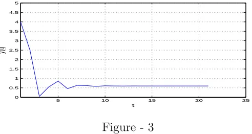
Example 3.3. For ν = 3, δ = 5, µ = 2 and = 3, y−1 = 4, y0 = 2.5, we get y21 = 0.7862<4.
t 0 1 2 3 4 5 6 7
Y(t) 4.0007 2.5000 0.0086 0.2267 2.6777 0.3632 0.1382 1.4022
t 8 9 10 11 12 13 14 15
Y(t) 0.7160 0.2164 0.7436 0.9879 0.3712 0.4575 0.9832 0.5587
t 16 17 18 19 20 21 22 23
Y(t) 0.3866 0.7842 0.7219 0.4291 0.5995 0.7862 0.5237 0.5059
Figure - 1
Theorem 3.4. Let δ > ν and
δ
− (2δµ−νµ) ln ν(ν−δ)(ln+ 2)−2δ2ln
<
µ+((ν+δ) ln−δ)(2δµ−νµ) ln
ν(ν−δ)(ln+ 2)−2δ2ln
ln. (10)
Then, the equilibrium point y >¯ 0 of (1) is locally asymptotically stable.
Proof. From Definition 2.2, we get the linearized equation and the characteristic
equation associated with (1) about ¯y is
yt+1+
ν(−¯y + ¯y)
(µ+ (ν+δ)¯y) lnyt+
δ(−¯y+ ¯y)
(µ+ (ν+δ)¯y) lnyt−1 = 0, n∈N(0) (11)
and
µ2+ ν(
−¯y+ ¯y)
(µ+ (ν+δ)¯y) lnµ+
δ(−¯y+ ¯y)
(µ+ (ν+δ)¯y) ln = 0, (12)
respectively. From Theorem 2.3 we obtain
− ν(
−¯y+ ¯y) (µ+ (ν+δ)¯y) ln
<1 + δ(
−¯y+ ¯y)
(µ+ (ν+δ)¯y) ln <2. (13)
We derive
−¯y < (µ+ (ν+δ)¯y) ln−δy¯
b , (14)
−¯y < (µ+ (ν+δ)¯y) ln
ν−δ −y¯ (15)
and
−¯y < 2(µ+ (ν+δ)¯y) ln−νy¯
(15)⇒ (ν−δ)¯y <(µ+ (ν+δ)¯y) ln+ (δ−ν)−¯y. Substituting (16), we get
¯
y < (2δµ−νµ) ln
ν(ν−δ)(ln+ 2)−2δ2ln.
Again substituting in (14), we get
δ
− (2δµ−νµ) ln ν(ν−δ)(ln+ 2)−2δ2ln
<
µ+ ((ν+δ) ln−δ)(2δµ−νµ) ln
ν(ν−δ)(ln+ 2)−2δ2ln
ln.
Example 3.5. For ν = 3, δ = 5, µ = 2, = 3 and condition (10) of the Theo-rem 3.4 does not hold, then every positive equilibrium solution of (1) is not locally
asymptotically stable.
5 10 15 20 25
0 0.1 0.2 0.3 0.4 0.5 0.6 0.7 0.8 0.9 1 t y(t)
Figure - 2
Theorem 3.6. (i). Equilibrium solution y¯is nonrepeller.
(ii). Equilibrium solution y¯is not a saddle point.
(iii). Equilibrium solutiony¯is a nonhyperbolic point when a≤2b.
Proof. (i). From (12) and from Theorem 2.3 (iv), we get
δ(−¯y + ¯y) (µ+ (ν+δ)¯y) ln
>1 (17)
and
ν(−¯y + ¯y) (µ+ (ν+δ)¯y) ln
<
1− δ(
−¯y+ ¯y) (µ+ (ν+δ)¯y) ln
Substituting (17) in (18) we getν <0 which contradicts our assumption thatν > 0.
Thus the equilibrium solution ¯y is nonrepeller.
(ii). From (12) and from Theorem 2.3 (v), we get
(µ+ (ν+δ)¯y) ln > −ν
2(−¯y + ¯y)
4δ (19)
and
ν(−¯y + ¯y) (µ+ (ν+δ)¯y) ln
>
1− δ(
−¯y+ ¯y) (µ+ (ν+δ)¯y) ln
. (20)
Substituting (19) in (20) we get 4νδ > ν2+ 4δ2.
This is not possible since ν >0 and δ >0 are constants. Therefore, no equilibrium
solution is a saddle point.
(iii). From (12) and from Theorem 2.3 (vi), we get
(µ+ (ν+δ)¯y) ln=−δ(−¯y+ ¯y) (21)
and
ν(−¯y + ¯y) (µ+ (ν+δ)¯y) ln
≤2. (22)
Substituting (21) in (22) we get ν <2b.
Example 3.7. For ν = δ = µ and for = 2 we get equilibrium solution ≈ 0.65 which is a nonhyperbolic point.
5 10 15 20 25
0 0.5 1 1.5 2 2.5 3 3.5 4 4.5 5 t y(t)
4
Conclusion
In this paper, we discuss the different characters like periodic, stability and
boundedness of the solutions of the rational exponential difference equation (1).
Earlier results exist for similar type of difference equation when the independent
variable is raised as a power of e. Here we have generalized the results when the
independent variable is raised to any >1. Earlier results are available only on the
study of the stability of the solutions but, we have analyzed more characters like
boundedness and the asymptotic behavior of solutions of the equation (1) which is
new in the literature. Suitable examples are provided to validate our results and
they are verified with MATLAB.
Author contributions
All authors contributed equally and the all authors have read and agreed to the
present version of the manuscript.
Funding
This research received no external funding.
Conflicts of interest
The authors declare no conflict of interest.
References
[1] A.M.Ahmed, A.G.Sayed and Waleed Abuelela,On Globally Asymptotic Stability
of a Rational Difference Equation, Southeast Asian Bulletin of Mathematics,
[2] L. Berg and S. Stevic,On the Asymptotic of some Difference equation, Journal
of Difference Equations and Applications, 18(5) (2012), 785 – 797.
[3] Fatma Bozkurt, Stability Analysis of a Nonlinear Difference equation,
Interna-tional Journal of Modern Nonlinear Theory and Application, 2 (2013), 1 – 6.
[4] Elias Camouzis and G. Ladas, Dynamics of Third Order Rational Difference
Equations with Open Problems, Chapman & Hall/CRC, 2007.
[5] R. De Vault, W. Kosmala, G. Ladas and S.W. Schultz,Global Behavior ofyn+1 = p+yn−k
qyn+yn−k
, Nonlinear Analysis, 47(2001), 4743 – 4751.
[6] D.S. Dilip, Adem Kilicman and Sibi C.Babu, Asymptotic and Boundedness
Be-havior of a Rational Difference Equation, Journal of Difference Equations and
Applications, doi.org/10.1080/10236198.2019.1568424.
[7] V.V.Khuong and T.H.Thai, On the Recursive Sequence xn+1 =
αxn−1 βxn+xn−1
+
xn−1 xn
, Southeast Asian Bulletin of Mathematics, 41(2017), 37 – 44.
[8] M. Kulenovic and G. Ladas, Dynamics of Second Order Rational Difference
Equations, Chapman & Hall/CRC, 2002.
[9] Longtu Li,Stability Properties of Nonlinear Difference Equations and Conditions
for Boundedness, Computers and Mathematics with Applications, 38 (1999), 29
– 35.
[10] Levi.D, Termblay. S, Winterniz. P,Lie point symmetries of difference equations
and lattices. J.Phys. AMath. Gen. 33 (2001), 8501–8523.
[11] Levi. D, Termblay. S, Winterniz. P,Lie symmetries of multidimensional
differ-ence equations. J. Phys. A Math. Gen. 2001, 34, 9507–9524.
[12] Levi. D, Winterniz. P,Continuous symmetries of difference equations. J. Phys.
[13] H. El-Metwally, E.A. Grove, G. Ladas, R. Levins and M. Radin, On the
Dif-ference Equation xn+1 = α+βxn−1e−xn , Nonlinear Analysis, 47(2001), 4623 –
4634.
[14] C.H.Gibbons, M.R.S Kulenovic, G.Ladas, H.D Voulov,On the trichotomy
char-acter of xn+1 =
(α+βxn+γxn−1) A+xn
, Journal of Difference Equations and
Appli-cations, 8(1)(2002), 75 – 92.
[15] V.L.Kocic and G.Ladas,Global Behaviour of Nonlinear Difference Equations of
Higher Order with Applications, Kluwer Academic Publishers, Dordrecht, 1993.
[16] S.A.Kuruklis, The asymptotic stability of xn+1−axn+bxn−k = 0, Journal of Mathematical Analysis and Applications, 188 (1994), 719 – 731.
[17] W.Kosmala, M.R.S Kulenovic, G.Ladas, C.T. Teixeira, On the recursive
se-quence yn+1 =
p+yn−1 qyn+yn−1
, Journal of Mathematical Analysis and applications,
2(200), 571 – 586.
[18] W.S He, W.T. Li,Attractivity in a nonlinear delay difference equation, Applied
Mathematics, E-Notes 4(2004), 48 –53.
[19] I. Ozturk, F. Bozkurt and S. Ozen, Global Asymptotic Behavior of the
Dif-ference Equation yn+1 =
αe−(nyn+(n−k)yn−k) β+nyn+ (n−k)yn−k
, Applied Mathematics Letters,
22(2009), 595 – 599.
[20] I. Ozturk, F. Bozkurt and S. Ozen,On the Difference Equation yn+1= α+βe yn
γ+yn−1, Applied Mathematics and Computation, 181 (2006), 1387 – 1393.
[21] G. Papaschinopoulos, C.J. Schinas and G. Ellina, On the Dynamics of the
So-lutions of a Biological Model, Journal of Difference Equations and Applications,
20(5 - 6) (2014), 694 – 705.
[22] D. Tilman and D. Wedin,Oscillations and Chaos in the Dynamics of a