Mathematical modeling of planar and spherical vapor–liquid phase interfaces
for multicomponent fluids
David Celn´y1,2,a, V´aclav Vinˇs1, Barbora Plankov´a1,2, and Jan Hrub´y1
1 Institute of Thermomechanics, of the CAS, v. v. i., Dolejˇskova 1402/5, Prague, Czech Republic
2 Faculty of Nuclear Sciences and Physical Engineering, Czech Technical University in Prague, Bˇrehov´a 78/7, Prague, Czech Republic
Abstract. Development of methods for accurate modeling of phase interfaces is important for understanding various natural processes and for applications in technology such as power production and carbon dioxide separation and storage. In particular, prediction of the course of the non-equilibrium phase transition processes requires knowledge of the properties of the strongly curved phase interfaces of microscopic droplets. In our work, we focus on the spherical vapor–liquid phase interfaces for binary mixtures. We developed a robust computational method to determine the density and concentration profiles. The fundamentals of our approach lie in the Cahn-Hilliard gradient theory, allowing to transcribe the functional formulation into a system of ordinary Euler-Langrange equations. This system is then split and modified into a shape suitable for iterative computation. For this task, we combine the Newton-Raphson and the shooting methods providing a good convergence speed. For the thermodynamic properties, the PC–SAFT equation of state is used. We determine the density and concentration profiles for spherical phase interfaces at various saturation factors for the binary mixture of CO2and C9H20. The computed concentration profiles
allow to the determine the work of formation and other characteristics of the microscopic droplets.
1 Introduction
The phase interface is the layer separating bulk thermodynamic phases, the liquid and the gas phases in the present case. The thickness of the phase interface is typically on the order of nanometres. Yet, understanding the physics of vapor-liquid phase interfaces is important for numerous natural processes and applications in technology. In particular, the present study aims at modeling the phase transition phenomena in systems relevant for carbon capture and storage technologies. The subject of interest of this study are microscopic droplets, whose diameter is comparable with the thickness of the phase interface. Such droplets occur in the process of nucleation of a liquid phase from the metastable supersaturated gas phase.
The phase equilibrium state of the system has to be investigated first. For this purpose, an equation of state (EoS) is needed. The usual approach is to choose one of the simple low parameter equation (Van der Waals, Redlich-Kwong, Peng-Robinson or their modifications). Here we employed an advanced PC-SAFT EoS. This equation belongs to a family of EoSs derived from the statistical fluid association theory (SAFT) [1]. The perturbed chain modification PC-SAFT was developed by Gross and Sadowski [2]. Various approaches are available to characterize the phase interface. The Gibbsian approach, treating the phase interface as infinitesimally
a e-mail::celnydav@fjfi.cvut.cz
thin, allows to properly describe the integral properties of the phase interface such as the surface tension, molecular adsorption and related thermodynamic properties. However, it does not provide a tool to predict the dependence of the surface tension on composition of the adjacent phases and on the curvature of the phase interface. The so-called capillarity approximation, which is one of the main assumptions of the classical nucleation theory (CNT) [3], assigns properties of the macroscopic planar phase interface to the strongly curved interface of the microscopic droplets. Modeling the effect of the surface curvature is possible with the gradient theory(GT) [4, 5] or density functional theory (DFT) [6]. These theories enable to obtain the density profiles (dependence of the local density on the coordinate perpendicular to the surface) and other characteristics of the phase interface.
This study is a continuation of the research of phase interfaces using GT previously done by Hrub´yet al. [7, 8] and Plankov´a [9]. In this work, we propose a new approach to the mathematical solution of the problem obtained from GT. This solution is iterative and offers a way of splitting the problem into two consecutive steps that can be solved separately.
2 The modeled system
We consider an n-component mixture (two components in this study) in the state of metastable supersaturated gas C
phase. We consider a microscopic droplet in the thermal and chemical equilibrium with the gas phase, meaning that the temperature and chemical potentials are homogeneous throughout the system. The modeled droplet corresponds to the so-called critical cluster of the molecular theory. We note that the opposite situation with a bubble in the equilibrium with a superheated or stretched liquid would be very much alike.
When the system is composed of two components, the phase equilibrium state with a planar phase interface can be easily computed for the given temperatureT and pressure p based on the conditions of thermodynamic equilibrium of the liquid and gaseous phases: equality of temperatures, chemical potentials for both components, and equality of pressures in both phases. As a result, we obtain the densities and compositions of both phases.
To proceed from the system with a planar phase interface to the system with a droplet, we increase the concentration of the less volatile component (here n-nonane) in the mother phase (gas) by multiplying it by the saturation ratioα > 1, while keeping the concentration of the more volatile component (carbon dioxide) and temperature constant. The saturation ratio directly influences the size of the droplet: a bigger saturation ratio results in a smaller droplet. We note that choosing a too high saturation ratio might result into an unstable state (a state beyond the vapor-liquid spinodal). For the supersaturated gas phase obtained in this way, we determine the liquid phase in thermal and chemical equilibrium. From the condition of equality of chemical potentials of each components in both phases we determine the concentrations of the components in the liquid phase and the corresponding pressure of the liquid phase, which is bigger than for the mother gas phase. The magnitude of difference is also directly influenced by the saturation factor in a manner that higherαmeans higher pressure difference. The thermodynamic state of the liquid obtained in this way is the state of idealized liquid droplet in the Gibbsian picture. The difference of pressure is related to the Laplace pressure due to the surface tension of the curved interface. The “equilibration” of the droplet with the gas phase is iterative process. The iteration is continued even a few steps after the stop criterion is reached and the best result is chosen among the computed after-steps. The purpose of this measure is avoiding wrong results due to premature termination of the iteration.
The thermodynamic state obtained in this way is hypothetical because even the center of the droplet is influenced by the phase interface. However, the density and concentrations obtained in this way are used to provide the first guess of local conditions in the center of the droplet in the gradient theory modeling.
3 Gradient theory
The gradient theory, also called Cahn-Hilliard theory [4], was developed by Cahn and Hilliard in 1957, although its foundations were already given by van der Waals. The basis of the GT is an expansion of the Helmholtz energy into a Taylor series with respect to the gradient of density or gradients of concentrations. This expansion is then used to obtain the grand potential of the system, which is treated as
a functional of the density or concentration profiles. These profiles are then determined by minimizing the functional, or more precisely, finding its stationary point by solving the corresponding Euler-Lagrange (E-L) differential equations.
In this study, we define the functional as the work of formation given by Eq. (1):
W =Ωinhom−Ωhom. (1)
Here, Ω is the grand potential. The subscripts in this equation indicate homogeneous system (only the gaseous mother phase) and inhomogeneous system (system including a droplet with some gaseous surroundings at the same temperature and chemical potentials).
The grand potentialΩcan be expressed in terms of the Helmholtz free energy of the inhomogeneous system. The form of the functional can be transformed into the spherical coordinates. The changed coordinate system allows using the symmetry of spherical droplet and simplifies the expression into the following form:
W =
R
0
⎛ ⎜⎜⎜⎜⎜
⎜⎝Δω(ρ(r))+1 2
n
i,k=1
ci,k(∇ρi(r)) (∇ρk(r))
⎞ ⎟⎟⎟⎟⎟ ⎟⎠4πr2dr.
(2) We can see from Eq. (2) that integral is one dimensional and all concentrations ρi depend on the radial coordinate only. ci,kin Eq. (2) denotes the so-called influence parameter. And the termΔωis a composite of the Helmholtz energy density and termiρiμi. Also this term depends on density profile functionρ(r). We denote density profile function in a vector shape because it is composed of concentration profiles for both components.
For given density profile the functional (2) returns the work needed to form an inhomogeneity represented by this density profile. Our task is now to obtain the most probable density profile for the given system conditions. Such demand according to the paper [4] requests a minimization of the formation work. The solution yields saddle point and minimal points of functional W. We are interested only in the saddle point because it corresponds to the required density profile for the droplet. The minimum points on the other hand represent a homogeneous system (gaseous or liquid) without any phase interface.
The saddle point is found using E-L system of two second order differential equations Eq. (3):
∂W ∂ρk−
d dr
∂W ∂ρ k
=0,k∈1. . .n. (3)
Whereρdenotes differential ofdρ/dr. Expressing the work of formation in Eq. (3) in terms of the GT, we obtain Eq. (4):
n
i=1 ci,k
2 rρ
i+ρi
=Δμk,k∈1. . .n. (4)
interaction of components ci,k as a geometric mean of the influence parameters for the pure components √ci,i·ck,k:
n
i=1 √
ci,i
2 rρ
i+ρi
= √Δμk ck,k,k∈
1. . .n. (5)
Eq. (5) is the basis for the present computations. Various methods can be developed to solve this equation. The present method provides benefits of substantial speed-up, modifiability of computation and result precision.
4 Solution of the Euler-Lagrange equations
Our method uses elementary results of the gradient theory and modifies it into a two step iterative method. We notice the similarity in right hand side of equation within Eq. system (4) and subtract the first equation from the others. This operation gives us system composed of one differential equation (6) and n−1 non-linear algebraic equations (7). For our case is j∈2. . .n.
n
i=1 √
ci,i
2 rρ
i+ρi
= √Δμ1 c1,1
, (6)
Δμj √
cj,j = Δμ1 √
c1,1.
(7)
This system contains equations coupled through their right-hand sides. Our goal is to split the solution into solving algebraic part (7) and the differential part (6) separately. To ensure that these equations are coupled, the algebraic part (7) has to be solved first. Then, its results are used in the computation of equation (6). We perform a special substitution:
˜ ρ=
n
i=1 √
ci,iρi n
i=1 √
ci,i .
(8)
The substitution transforms the components concentrations ρi into modified molar density ˜ρ. Substitution also ensures simple shape of E-L equations and enable discretization. We can also see that shape of substitution (8) is invariable to differentiationd/dr. This feature of ˜ρis used in differential equation. Secondly, a new artificial variable X is inserted. To clarify the dependence in system of Eq. (7, 6) we choose X=−Δμ1/√c1,1. For j∈2. . .nwe then obtain a system:
⎛ ⎜⎜⎜⎜⎜ ⎝
n
i=1 √
ci,i
⎞ ⎟⎟⎟⎟⎟ ⎠
2 rρ˜
+ρ˜=−X, (9)
Δμj √
cj,j
=−X. (10)
This system (9,10) is basis of following computation. The solution of equation (9) is possible only with the knowledge of artificial variableXin the molar density interval. For that purpose X has to be computed. The dependence of X variable enables the discretization of ˜ρ across the molar density interval. At these discretized points we compute values ofX.
4.1 Solution of the algebraic equations
As the first step we take only algebraic part (10). The artificial variableXallows to rewrite the algebraic part into a system of similar algebraic equations. As a result of adding new variable, one new equation also needs to be appended. The last equation is provided by definition (8). This completes the analytic system of equations (11). , where for j∈2. . .nwe have:
Δμ1(ρ) √
c1,1 +X= 0 ... ... ... Δμn(ρ)
√
cn,n +X= 0
n
i=1 √
ci,iρi n
i=1 √
ci,i − ˜
ρ=0. (11)
The system (11) needs to be solved for values ofXandρat each point of discretization. This provides the function dependence sampled across the molar density interval. Results of each iteration X( ˜ρi), ρ( ˜ρi) are saved into data matrix M1. The secondary computational data (dX( ˜ρi)/dρ˜, dρ( ˜ρi)/dρ˜) are also saved into data matrix M2. The data matrices are useful in post-processing phase for computation of approximate of requested functionsXandρ. To solve this system the Newton-Raphson iterative method is used. For sufficiently fine division (500 points or more for best performance) the iteration is commenced. The Newton-Raphson method requires to compute the Jacobian of system (11) and sufficient first estimate. First guess for boundary points is provided by boundary conditions of system that we obtained from supersaturated equilibration. And points inside discretization use previous result as their first estimate. Owing to the fine discretization, the solution for each point is found in two to five Newton-Raphson iterations.
When the computation is completed, the obtained matrices M1 andM2 are used to compute piecewise cubic approximation of functions X( ˜ρ), ρ1( ˜ρ), and ρ2( ˜ρ). Examples of these functions for saturation ratioα=1.5 are shown in figures 1 and 2. For each point of discretization except the first we compute coefficients for cubic polynomial with function values from M1 and with derivatives from the M2. The three piecewise cubic curves then provide a link between the two parts of the problem and are used for the solution of differential equation.
4.2 Solution of the differential equation
/
Fig. 1. FunctionX( ˜ρ) computed by solving system of equations
(11) for saturation ratio 1.5.
/
Fig. 2. Dependencies of the concentrations ρ1 and ρ2 on the
modified density ˜ρcomputed by solving system of equations (11) for saturation ratio 1.5
the derivative of the modified density is also zero as a consequence of the spherical symmetry.
The solution method is based on the decomposition of the second order equation into system of two first order equations. The boundary problem is then solved by a shooting method, converting the boundary problem into the initial one. Our shooting parameter is the initial modified liquid density ˜ρ0. The solution of the initial problem is computed with solving method ODE45, which is Runge-Kutta (4,5) method within MATLAB(R)libraries. As an option we requested to stop the computation either when the computed modified density reaches a negative value or its derivative equals zero.
The next value of shooting parameter is computed using the bisection method. At first the profile is computed for initial shooting parameter. The minimal value ˜ρmin of the profile is found and applied for the decision of the next shooting parameter ˜ρ0.
We use the robust decision criteria that takes only minimal value of the profile ˜ρmin into account. If the ˜ρmin value is below the ˜ρG level then lower shooting parameter
˜
ρ0is needed. Similarly, when ˜ρmin is above the gas density level ˜ρG, the higher shooting parameter ˜ρ0is chosen.
The iteration continues until specified precision is reached, or size of the interval is below numeric precision of double number format. When the iteration terminates successfully, the profile found this way is denoted as result profile and shooting parameter as ˜ρ0,res.
5 Results
We implemented the splitting method and computed the density profiles for the system of carbon dioxide CO2 and n-nonane C9H20. The phase equilibrium system conditions were set to T = 350 K and p = 10 MPa. The saturation factor alpha for this system was determined to range from α∈ 1.15,4.
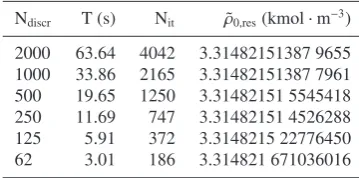
The discretization constant for the algebraic solution was set to 1000 points inside intervalρG,˜ ρL˜ . This option provided enough division points during the iteration and accurately use the interpolation. Performed analysis shows that the discretization interval can be chosen even ten times smaller, still providing accurate results. This fact is illustrated in table 1 and is caused by the efficiency of the piecewise cubic interpolation.
As problematic appear areas outside of the modified density interval. Here, extrapolation is used which is sensitive to errors in interpolation coefficients. However, extrapolation is only used for initial iteration or for unphysical profiles which might occur during the iteration. The result profile does not suffer from the extrapolated data. Table (1) illustrates also the iteration dependency. Rough discretization have the average ratio of iteration per point around 3:1 but as the refinement increases the iteration ratio changes to 2:1. This nicely correspond to section section Algebraic solution where this behaviour was explained. The last column of table represent precision of result profile initial condition computation. The initial condition is our shooting parameter and we expect it to improve as the refinement of discretization improves. The space in values is inserted for clarity reasons at position of first different digit.
Table 1.Comparison of algebraic solution for different number of
discretization points. Ndiscris the number of discretization point,T
is required time of computation, Nitshow how many iterations were
performed and ˜ρ0,resis the found result profile initial condition
Ndiscr T (s) Nit ρ˜0,res(kmol·m−3)
2000 63.64 4042 3.31482151387 9655 1000 33.86 2165 3.31482151387 7961 500 19.65 1250 3.31482151 5545418 250 11.69 747 3.31482151 4526288 125 5.91 372 3.3148215 22776450 62 3.01 186 3.314821 671036016
circle line and black full line) from figure 3 correspond to physical reality. The cyan square line depicts the convergence of solution to a thermodynamically unstable state that is also a valid solution. The other lines (green cross line and magenta triangle line) represent the non-physical solutions, where extrapolation of data from algebraic solution are used. These profiles quickly escapes the interesting region and are immediately truncated during computation.
/
Fig. 3.Modified density profiles for different values of shooting
parameter ˜ρ0with saturation factorα=1.5. Black profile denoted
as ˜ρ0,optis result profile.
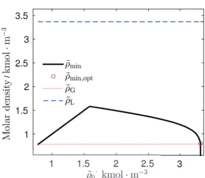
The search for optimal starting condition exhibits interesting behavior when approaching the optimal value. This behavior is captured in figure 4. Compared to previous figure, we plot only the dependency of found minimum of the density profile on initial modified density. The black full line from figure 4 is composed of two segments. A linear segment and a “logarithmic” segment. The linear segment is of no importance because it only illustrate the incrementation of the initial condition ˜ρ0. The interesting situation happens for the logarithmic segment. This segment represents the search for optimal value of initial condition that is further used as result.
We know that the optimal profile is the one with minimum value equal to the modified gas density ˜ρG and, because of that the optimal profile is found at the intersection with the red dotted line on figure 4 representing
˜
ρG. Before this value we find profiles similar to cyan square line from previous figure 3 that snap to thermodynamically unstable solution. And after magenta circle we see rapid descend into negative region of figure that corresponds to the green cross line from previous figure 3. This is the reason for decision criteria to evaluate the minimal values of profiles. Because of this feature we are able to distinguish the small details, where the profile changes from cyan square line into green cross line. This is the moment we are looking for and even small variation in the initial condition influence the profile dramatically.
The common problem of such behaviour is the precision of double number format. Available range of representable numbers is not sufficient for capturing optimal profile. The
/
Fig. 4.Minimal value of modified density profile ˜ρmindependence
on values of shooting parameter ˜ρ0with saturation factorα=1.5.
Magenta circle denoted as ˜ρmin,opt is found minimum for result
profile.
profile is suboptimal and display only small region where it satisfy the right boundary condition ˜ρopt = ρG˜ . The use of other number format would not solve the problem only extend the range of computable profiles. We have not performed the reimplementation into more precise number format because double is the greatest number type natively supported by MATLAB environment. The variable precision that is supported by minority of MATLAB function is also unacceptable due to is poor performance which would cause overall slowdown of computation.
For the reasons given above we chose the initial conditions in the safe region and perform computation there. We computed specified profile for three saturation factors of α ∈ {4,1.5,1.15} respectively to illustrate the growth of the droplet with decreasing saturation factor. With the modified density ˜ρ used in our computation and comparison of results we also computed components densities ˜ρ1 and ˜ρ2 that correspond to CO2 and C9H20 respectively. The boundary conditions were also included.
In our first system depicted in figure 5 we notice that only small droplet is formed. Due to the high saturation factor, the gas density is noticeably higher compared to figures 6 and 7. This figure also illustrates the droplet with no bulk liquid content. The droplet is so small in diameter that only phase interface is present. This fact is denoted by the density profile (black full line) that does not reach the blue dashed line ˜ρL.
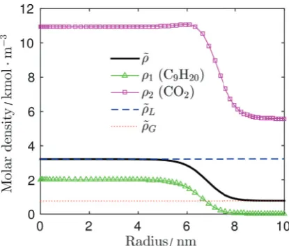
The second system in figure 6 captures a small droplet with nearly no liquid content. This figure corresponds to the saturation factor ofα=1.5 and show interesting behavior of carbon dioxide. Carbon dioxide adsorbs at phase interface. It means that its molecules accumulate at the phase interface and density profile than have small peak within the phase interface. This behavior is noticeable also in figure 7.
/
Fig. 5. Modified density profile and partial densities profiles
(concentration) for the saturation factorα=4.
/
Fig. 6. Modified density profile and partial densities profiles
(concentration) for the saturation factorα=1.5.
/
Fig. 7. Modified density profile and partial densities profiles
(concentration) for the saturation factorα=1.15.
precision of computation. This error is most significant for bigger droplets with high ratio of pure liquid compared to phase interface. This problem is currently being solved with use of an analytical solution near zero radius.
6 Conclusion
Of the various approaches to the phase interface modeling, the gradient theory provides a good compromise between the physical detail and mathematical tractability. For this theory we developed a new solution method for multi-component mixtures and tested it for a binary system. In this work we presented the main steps of the method and offered information on variable parameters. We have also highlighted the problematic areas of computation which primarily concern very large droplets with almost “top hat” density profile.
Acknowledgement
We gratefully acknowledge the support by Grant No. GAP101/11/1593 of the Czech Science Agency, Grant No. 7F14466 of the Czech-Norwegian Research Programme CZ09 and institutional support RVO:61388998.
References
1. W. Chapman, K. Gubbins, G. Jackson, M. Radosz, Fluid Phase Equilib.52, 31 (1989)
2. J. Gross, G. Sadowski, Ind. Eng. Chem. Res. 40, 1244 (2001)
3. Y. Drossinos, P.G. Kevrekidis, Phys. Rev. E: Stat., Nonlinear, Soft Matter Phys.67(2003)
4. J.W. Cahn, J.E. Hilliard, J. Chem. Phys.28, 258 (1958) 5. J.W. Cahn, J.E. Hilliard, J. Chem. Phys.31, 688 (1959) 6. J. Gross, J. Chem. Phys.131(2009)
7. J. Hrub´y, D.G. Labetski, M.E.H. van Dongen, J. Chem. Phys.127, 164720 (2007)
8. J. Hrub´y, B. Plankov´a, V. Vinˇs, Corrections to the classical work of formation of critical clusters, inNucl. and Atmos. Aerosols: 19th Int. Conf. (AIP Publishing LLC, 2013)