Type of the Paper (Article.)
1
The zeros of the Dirichlet Beta Function encode the
2
odd primes and have real part 1/2
3
Anthony Lander
4
Birmingham Women’s and Children’s Hospital NHS Trust, Birmingham UK; [email protected]
5
Tel.: 0121 333 9999
6
7
Abstract: It is well known that the primes and prime powers have a deep relationship with the
8
nontrivial zeros of Riemann’s zeta function. This is a reciprocal relationship. The zeros and the
9
primes are encoded in each other and are reciprocally recoverable. Riemann’s zeta is an extended or
10
continued version of Euler’s zeta function which in turn equates with Euler’s product formula over
11
the primes. This paper shows that the zeros of the converging Dirichlet or Catalan beta function,
12
which requires no continuation to be valid in the critical strip, can be easily determined. The
13
imaginary parts of these zeros have a deep and reciprocal relationship with the odd primes and
14
odd prime powers. This relationship separates the odd primes into those having either 1 or 3 as a
15
remainder after division by 4. The vector pathway of the beta function is such that the real part of its
16
zeros has to be a half.
17
Keywords: Catalan beta function; Riemann’s zeta function; primes; Dirichlet L-function
18
19
1. Introduction
20
Euclid’s lemma, states that if is prime and | , where and are integers then | or
21
| [1]. This leads us to the Fundamental Theorem of Arithmetic (FTA) that every ∈ ℕ is the
22
product of a unique set of primes, each prime being raised to a specific power;
23
= … , where = 2, = 3, = 5, … ∈ ℙ and , ,…∈ ℕ . (1)
Euler’s zeta function equates to Euler’s product formula over the primes and this encodes the FTA;
24
( ) = = (1 − )
= (1 + + + ⋯ ) with ∈ ℝ.
(2)
This important relationship is easily extracted by multiplying out the right-hand side of Equation
25
(2);
26
( ) = 1 + + + + + + + + + + ⋯. (3)
Euler’s Zeta converges when > 1 but Riemann’s zeta ( ), with ∈ ℂ, is in a form that “remains
27
valid for all ”. Riemann sought to extend Euler’s zeta in analogy to the well-known extension of the
28
factorial function for > −1 in Γ( + 1) = lim
→ ( + 1)
. . …
( )( )( )…( ).
29
Riemann’s derivation of ( ) substitutes for in the integral Γ( + 1) = ∫ to
30
give Γ( ) = ∫ for > 0, ∈ ℕ . This is then summed over to give
31
Γ( ) ∑ = ∫ ( − 1) for > 1. Riemann proceeds with a contour integral expressed
32
as ∫ ( ) . This integral is considered to run down a line just above the positive real axis before
33
circling the origin anticlockwise, and then running back up a line just below the positive real axis.
34
Then, after some manipulation, zeta is defined by ( ) = ( )∫ ( ) which for real values,
35
= , returns Euler’s zeta ( ) = ∑ [2].
36
The number of primes less than , designated ( ), is asymptotic to /ln( ). This relationship
37
was conjectured by Gauss in the 1790’s and proved by Hadamard [3] and de la Vallée Poussin in
38
1896 [4]. The relationship is known as the Prime Number Theorem and makes use of Riemann’s
39
famous paper of 1859 entitled “On the Number of Primes Less Than a Given Magnitude” [5].
40
Riemann’s explicit formula for ( ) = lim
→ ( + ) + ( − ) 2⁄ is given in terms of
41
Π ( ) which counts the primes and prime powers up to , counting a prime power as 1/ of a
42
prime;
43
Π ( ) = ⁄ . (4)
The Möbius function ( ), is related to the inverse of ( ) being 1⁄ ( )= ∑ ( ) , which
44
enables the number of primes to be recovered, ( ) = ∑ ( ) Π ⁄ . Riemann’s formula
45
then becomes
46
Π ( ) = Li( ) − Li( ) − ln(2) + ( ( − 1) ln( )) . (5)
In Equation (5) Li( ) = ∫ (ln ( )) is the un-offset logarithmic integral and { } are the nontrivial
47
zeros.
48
Riemann’s hypothesis is that the Re( ) = 1 2⁄ for all for which there is ample evidence [6],
49
but no proof. The critical line is = 1/2 and it lies in the middle of the critical strip (0 < Re( ) < 1).
50
In 1914 Hardy [7] proved the infinitude of { } with = 1/2 for which large sets of the Im( ) are
51
now published [8]. Riemann’s zeta obeys the functional equation,
52
( ) = Γ(1 − )(2 ) 2 sin
2 (1 − ). (6)
Accepting the Riemann Hypothesis, the nontrivial zeros of Riemann’s zeta, ( ) = 0, with =
53
1 2⁄ + are captured in the set { }. It is then the set { } that has the deep relationship with all
54
primes. It is easy to show that Dirichlet’s eta function, which is an alternating zeta series
55
( ) = 1 − 2 + 3 − 4 + 5 … using = +
shares the set { } for its zeros (1 2⁄ + ) = 0.
56
Cognisant of the Riemann Hypothesis and reflecting on the famous Madhava-Leibniz series
57
4
⁄ = 1 − 1 3⁄ + 1 5⁄ − 1 7⁄ …, (7)
one is instantly inquisitive about the zeros of the alternating and converging series
58
( ) = 1 − 3 + 5 − 7 + 9 … using = + . (8)
Does ( ) = 0 require Re( ) = 1 2⁄ and does {Im( ) ∶ ( ) = 0} have an easily demonstrable
59
relationship with the primes? The series is known as the Catalan, or Dirichlet beta series. Empirically
60
the zeros of beta do sit on the critical line and we will index them with as , for which (1 2⁄ +
61
) = 0. Using for beta distinguishes these zeros from the for zeta.
62
The first aim of this work was to determine some zeros of the beta function by estimating the
63
value of beta on the critical line, seeking solutions of (1 2⁄ + ) = 0 over a range in .
64
The second aim was to locate a few zeros of beta through identifying “spikes” in the amplitude
65
of a wave generated by the odd primes themselves.
66
The third aim was to demonstrate that the zeros of beta can locate the odd primes and odd
67
prime powers; so examining the reciprocal relationship.
68
The third aim was to plot the vector pathway to convergence of the beta function and to
69
illustrate why its zeros require the Re( ) = 1 2⁄ .
2. Materials and Methods
72
Repetitive calculations were performed in Microsoft Excel with Visual Basic. GraphPad Prism 7
73
was used to prepare figures.
74
Let , ∈ ℙ the set of all primes, with ℙ = {2,3,5,7, … … }. The odd primes, using \ to mean
75
the set theoretic difference, is the set ℙ\{2} which we can separate into ℙ = { ∶ 4|( − 1)} =
76
{5, 13, 17, 29, 37 … } and ℙ = { ∶ 4|( − 3)} = {3, 7, 11, 19, 23, … }. Let , , ∈ ℕ and , , ∈ ℝ
77
with = √−1 so that ∈ ℂ and = + . Without causing confusion, will also be used to index
78
the nontrivial zeros in the set { }. Let the prime be the largest prime in an ordered subset of ℙ
79
and let be the largest natural in an ordered subset of ℕ .
80
This work aimed;
81
1. To estimate the values of early elements of the set { }, for which (1 2⁄ + ) = 0, up to some
82
convenient value of , by determining minima in (1 2⁄ + ) over a range of . The infinite
83
series were calculated to a convenient end point, see [9].
84
2. To prepare, by an alternative means, a subset of { } by using two subsets of odd primes, one
85
subset from ℙ and one from ℙ , and to compare these with values for { }, from (1) above.
86
3. To use the set { }, from (1), to confirm that it could locate the primes and prime powers of the
87
odd primes; anticipating that the primes would separate into those with residuals of 1 or 3 on
88
division by 4.
89
4. To illustrate that the vector pathway to convergence of the beta function can be equated to the
90
difference between two finite series whose behaviour, under changes in the real part of , limits
91
the zeros of beta to having real part a half.
92
3. Results
93
The relationship between { } and all primes, and the prime powers, is presented first to set the
94
scene, before turning to the relationship between { } and the two sets of odd primes and their
95
powers. The arguments for why the Re( ) = 1 2⁄ if ( ) = 0 follows from the pathway analysis.
96
3.1. Riemenn’s zeta: its nontrivial zeros and the primes
97
For zeta, we define an amplitude ( ) which we determine over a finite set of primes
98
{2,3,5,7, … … } and over the prime powers to a convenient limit . Our limit could be such
99
that < for all such that = ⌊ln( ) ln( )⁄ ⌋ for each , or we can let rise to some other
100
convenient ; the limit is not materially important in this illustration. Our amplitude is
101
( ) = ln( ) ( ⁄ )cos ln( ) . (3)
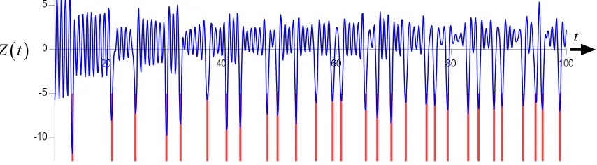
Using Equation (3), summating over the primes, and prime powers, to = 4409, the 600th
102
prime, and letting rise from 11 to 100, and letting = 20 generates Figure 1. Figure 1
103
incorporates red lines at the published values of the first 28 nontrivial zeros of zeta [8].
104
Z t
t
105
Figure 1. In blue the summated amplitudes of cosine functions, ln( ) ( ⁄ )cos ln( ), over a set
106
of primes and prime powers. In red, the first 28 elements of the set { }.
Using a subset of { }, the location of the primes , and the prime powers , can be recovered
108
over an interval in with ( ) to a convenient limit in of
109
( ) = cos ln( ) . (4)
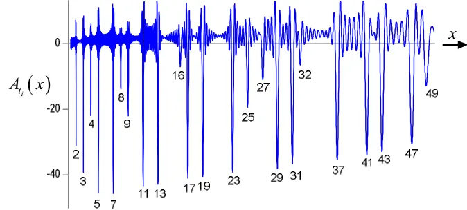
Using the first two hundred nontrivial zeros, = 200, we can recover the primes and prime powers
110
up to = 50 as shown in Figure 2.
111
i
t
A
x
x
112
Figure 2. The location of the primes and prime powers up to = 50 as determined from ( )=
113
∑=1cos ln( ) .
114
Having reminded ourselves of the deep reciprocal relationship { } ⇔ {ℙ} for zeta, we now
115
turn to the beta function.
116
3.2. The beta function and the odd primes
117
The beta function
118
( ) = (−1) (2 − 1) (5)
is also recognisable as a Dirichlet L-series defined as ( , ) = ∑ ( ) with the Dirichlet
119
character having modulus 4;
120
( , ) = ( ) modulus 4. (6)
Since all integers differ from a multiple of 4 by either 0, 1, 2 or 3, all the primes > 2 can be
121
placed into two groups; those where 4|( − 1) and those where 4|( − 3). Then in a similar way to
122
that in which Euler’s zeta ( ) = ∑ can be shown to equate to Euler’s product over the
123
primes ∏ in encoding the FTA, the beta series can be factorized as follows:
124
( ) = 1 − 3 + 5 − 7 + 9 …
3 ( ) = 3 − 9 + 15 − 21 + 27 …
(1 + 3 ) ( ) = 1 + 5 − 7 − 11 + 13 + 17 …
5 (1 + 3 ) ( ) = 5 + 25 − 35 − 55 + 65 + 85 …
(1 − 5 )(1 + 3 ) ( ) = 1−7 − 11 + 13 + 17 − 19 − 23 …
proceeding until it is clear that
125
( ) = 1
1 − ≡
1
1 + .
≡
(7)
In this way Dirichlet’s beta can be seen to have a relationship with the odd primes, ℙ\{2}.
The series has a Functional Equation [2]
127
(1 − ) = 2 π sin
2 Γ( ) ( ), (8)
and so if there is a zero at a with Re( ) = then, since we can ignore the sign of , there is also
128
a zero at Re( ) = for with 0 < < 1 2⁄ < and + = 1; reminiscent of the arguments
129
around the nontrivial zeros of ( ). Using ∈ ℕ a partial series ( ) has
130
Re ( ) = (−1) (2 − 1) cos( ln(2 − 1))
and Im ( ) = − (−1) (2 − 1) sin( ln(2 − 1)), (9)
which facilitate the plotting of the vector pathway in ℝ . We will denote this operation as P( ( ))
131
meaning the plotting of the vector pathway [9]. The pathway P( ( )) is then a plot of the
132
sequential vectors representing the partial series ( );
133
( ) = (−1) (2 − 1) and P ( ) ≡ ⃗
with the vectors ⃗ plotted in ℝ having
| ⃗| = (2 − 1) and arg( ⃗) = − ln(2 − 1) +
with = 0 if 2 ∤ and = if 2| .
(10)
The pathway has proximal and distal parts separated at a vector kappa. The distal pathway has
134
paired pseudo-spiral structures P(ℛ ) which can be counted from convergence in a retrograde
135
fashion starting with P(ℛ ). These structures have a principal-axis whose argument has a stability
136
under changes in which arises from a relationship with Euler’s spiral, see [9]. The magnitude of
137
the principal-axis of the P(ℛ ) is also derivable from the relationship with Euler’s spiral [9]. These
138
relationships allow the P(ℛ ) to be represented by novel vectors ℛ⃗ .
139
A positive integer , locates the ⃗ nearest the inflection point in the pathway of a smooth
140
curve that follows the final paired pseudo-spiral P(ℛ ) of P ( ) with
141
= 1 2
/ − 1 + 1 − / (11)
and that ⃗ will have a magnitude 2 − 1.
142
A second convergent vector series ℎ ( ) and its pathway of vectors P(ℎ ( )) summate an
143
ordered set of ℛ⃗ using the index to a final term of . A vector ℛ⃗ represents the magnitude of
144
the principal-axis of a P(ℛ ) and is an object in its own right. It has a magnitude ℛ⃗ being
145
ℛ⃗ = 2 − 1 (/ ) ( ), (12)
with an argument
146
arg ℛ⃗ = + ln 2 − 1 2 − 1
with = ⁄ if 4 2| and = 5 ⁄4 if 2 ∤ .
(13)
The parameter accounts for the alternating sign preceding each term of beta. The ⃗ faces
147
forwards for odd values and is reversed for even values. The series to terms, ℎ ( ) is defined as;
148
ℎ ( ) = ℛ⃗ with ℛ⃗ following ∈ ℕ ,
(14)
and the series ℎ ( ), to kappa terms is simply ℎ ( ) = ∑ ℛ⃗ .
We then have an approximation for the beta function as the difference between the two finite
150
series to kappa terms
151
( ) ≈ ( ) − ℎ ( ). (15)
This difference can be refined by taking account of the intersection of the ⃗ and ℛ⃗ with a
152
function = ( ̇) having ∈ { : 0 < ≤ 1} but whose finer details are not important. A vector
153
function closely related to ( ) which we will designate ( , ) is
154
( , ) = ( ) + ⃗ − ℎ ( ) + ℛ⃗ , (16)
whose symmetry breaking either side of = 1/2 is easily appreciated from P ( ) , P ( )
155
and P ℎ ( ) . It is this symmetry breaking which forces ( ) = 0 to have real part a half.
156
The pathway P ( ) has an ⃗ = ⃗ in the distal pseudo-spiral of its P(ℛ ) for which = ;
157
= / − 1 + 1 − / . (18)
The vector series P ( ) indexed by and P ℎ ( ) indexed by have proximal and distal
158
parts separated at terms designated kappa. A ⃗ for which = is designated ⃗ and a ℛ⃗ for
159
which = is designated ℛ⃗ . Kappa ∈ ℕ is defined as
160
= 1 2 (
/ − 1) / + 1 − / / . (19)
A residual, kappa dot written ̇ ∈ ℝ, with −1/2 ≤ ̇ ≤ 1/2 is simply,
161
̇ =1 2
/ − 1 / + 1 − / / − . (20)
Kappa dot is the domain of a function indicated = ( ̇) with 0 < ≤ 1 being the intersection of ⃗
162
and ℛ⃗ at the zeros.
163
A set of zeros of ( ) for ≤ 5250 at = 1 2⁄ were located by finding minima with very low
164
magnitudes in ( ), or at very low values of , using ( ); a sample appear in [9]. Intervals in
165
of 0.001 were examined from = 6 to = 4600 and then in intervals of 0.0001 from = 4600 to
166
= 5250. The zeros of beta from the set { } with ∈ ℕ being an index of the zeros of ( ). The
167
first 420 elements of { } appear in Table A1 in the Appendix.
168
Symmetrical pathways for a beta zero are illustrated in Figure 3.
169
170
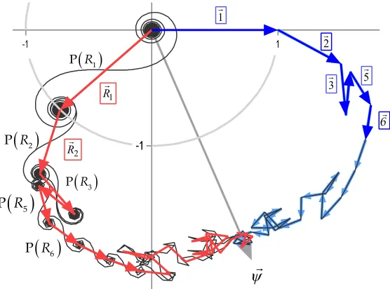
Figure 3. P (1 2⁄ + 5247.848260) for the 5944th zero of beta in black. In blue the P( ( )) with
171
= 29 with the first 6 vectors emboldened. In red P(ℎ ( )) retraces the distal P( ( )). The line of
172
reflection ⃗ is shown and P(ℛ ) to P(ℛ ) and P(ℛ ) and P(ℛ ) are labelled.
173
1P R
1
R
2
R
1
2
3
5
2 P R
3P R
5 P R
6 P R
Figure 3 shows a line of reflection ⃗ made of two rays ⃗ and ⃗ of unspecified magnitude
174
and having arguments and . The argument is
175
= arg ⃗ = ⁄ − ( 28 ⁄ )ln 2 − 1 . (17)
The principal argument is displaced clockwise from and so = − .
176
3.3. Symmetry breaking either side of = 1 2⁄
177
The terms “bigger” and “smaller” are used here to refer to the non-uniform enlargement and
178
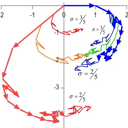
reduction of a pathway whilst accommodating differential scaling along that pathway. Figure 4
179
shows that for beta when < 1/2 the pathway P(ℎ ( )) is “bigger” than P( ( )), and when >
180
1/2 the pathway P(ℎ ( )) is “smaller” than P( ( )). This difference in behaviour is important
181
and underlies why there can be no zero when ≠ 1 2⁄ .
182
3 5
3 5
2 5
2 5
183
Figure 4. An illustration of how P ( ) and P ℎ ( ) change when rises or falls from 1 2⁄ .
184
Symmetry breaks differently either side of = 1 2⁄ . In green P ( ) and in orange P ℎ ( ) for
185
= 1 2⁄ . In blue P ( ) and in red P ℎ ( ) for two other values of as indicated.
186
The symmetry breaking evident in Figure 4 is consequent upon Equation (9) proximally, and
187
Equation (12) distally, see [9].
188
3.4. The beta function: its zeros and the odd primes
189
We now determine a subset of { } by summating cos ln( ) over a subset of the primes
190
and their lower powers. We define ( )
191
( ) = ln( ) ( ⁄ )cos ln( ) ℙ
− ln( ) ( ⁄ )cos ln( ) ℙ
(21)
Figure 5 and Figure 6 were prepared with 325 primes in each group having ℙ running from 5 to
192
= 4937, and ℙ running from 3 to = 4751 and allowing = 20.
B t
t
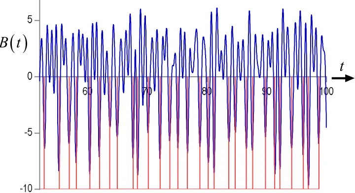
194
Figure 5. In blue is shown ( ) for 1 ≤ ≤ 52 prepared with Equation (21) using 325 primes in set
195
ℙ and 325 primes in set ℙ . In red are the first 21 zeros of ( ), see Table A1 (Appendix) these
196
collocate with the most negative minima in ( ).
197
The red lines in Figure 5 are zeros of beta from the set { } in Table A1 (Appendix).
198
B t
t
199
Figure 6. In blue is shown ( ) for 52 ≤ ≤ 100 prepared with Equation (21) using 325 primes in
200
each set ℙ and ℙ . In red are the 28 zeros from the 23rd to the 50th zeros of ( ), see Table 1
201
(Appendix); these collocate with the most negative minima in ( ).
202
Our next task is to see how well a subset of { } perform in ( ), with
203
( ) = cos ln( ) .
(22)
We anticipate that ( ) can identify and separate the odd primes. Figure 7 was prepared using
204
b tA
x
x
206
Figure 7. Shows positive spikes in ( ) coinciding with ∈ ℙ and with 3 and it is noted that
207
4|(3 − 1), whilst negative spikes coincide with ∈ ℙ and with 3 , 5 , 7 , 3 , 11 , 5 each of which
208
satisfies 4|( − 1).
209
Strictly, Figure 7 shows that [ ] ∈ ℙ rather than ∈ ℙ, but the localization of the centre of the
210
spikes to the integers is remarkably good and the errors are very small, (data not shown).
211
4. Discussion
212
The deep reciprocal relationship between the nontrivial zeros, { }, of Riemann’s zeta function
213
( ) and the distribution of the primes ℙ—accommodating all of its offspring as integral exponents
214
{ ∶ ∈ ℕ }—is beautiful, profound and well-known. The sets ℙ and { } are encoded in each
215
other—like the perfect marriage. Or are they? The literature often implies that the set { } is telling
216
ℙ how to behave—this is erroneous—the relationship is reciprocal, but the driver is ℙ. However, the
217
relationship is not monogamous.
218
This work shows that a similar reciprocal relationship connects the zeros of beta, { }, with the
219
distribution of the odd primes ℙ\{2} , accommodating all of its integral exponents { ∶ > 2, ∈
220
ℕ }, whilst dividing those primes and their offspring according to the remainder after dividing by 4.
221
The set ℙ\{2} and { } are entwined in each other—once ℙ drops its only even element—but
222
now ℙ\{2} has a relationship with the beautiful and spontaneously converging ( ).
223
The sets { } and { }, most likely, share characteristics, perhaps in the moments of the
224
distributions of the gaps between their elements, which could be of interest [9–13]. But it is also an
225
interesting question as to whether there is an encoded relationship between { } and { } which
226
ignores ℙ—this seems unlikely and ℙ may be quite happy about that.
227
The set ℙ remains prime.
228
229
230
231
232
233
Acknowledgments: This study was not funded. No funds have been received for covering the costs to publish
234
in open access.
235
Author Contributions: The author was the sole contributor.
236
Conflicts of Interest: The author declares no conflict of interest.
237
Appendix A
239
240
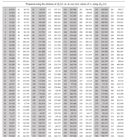
TABLE A1. Estimated zeros of (1 2⁄ + ): first 320
Prepared using the minima of ( ) or, at very low values of , using ( ).
1 6.0114 41 84.732 81 143.33 121 197.115 161 247.996 201 296.902 241 344.085 281 390.17 2 10.264 42 86.578 82 144.979 122 198.808 162 249.185 202 298.08 242 345.211 282 391.083 3 13.002 43 87.631 83 146.523 123 200.163 163 251.087 203 298.871 243 346.264 283 392.853 4 16.353 44 89.802 84 147.935 124 200.903 164 251.638 204 300.436 244 347.926 284 393.444 5 18.285 45 91.351 85 149.189 125 202.261 165 252.625 205 301.921 245 348.983 285 394.821 6 21.445 46 92.239 86 150.298 126 204.222 166 254.315 206 302.919 246 349.435 286 395.806 7 23.274 47 94.168 87 151.963 127 204.993 167 255.839 207 303.662 247 350.978 287 396.736 8 25.726 48 96.138 88 153.701 128 206.413 168 256.506 208 305.066 248 352.393 288 398.251 9 28.358 49 96.963 89 154.577 129 207.318 169 258.166 209 306.796 249 353.694 289 399.566 10 29.662 50 98.756 90 155.651 130 209.229 170 258.836 210 307.287 250 354.303 290 400.694 11 32.596 51 100.136 91 157.749 131 210.104 171 260.432 211 309.123 251 355.745 291 400.827 12 34.204 52 102.142 92 158.706 132 211.834 172 261.915 212 309.741 252 356.629 292 402.819 13 36.145 53 103.288 93 160.238 133 212.539 173 262.885 213 310.825 253 358.289 293 403.908 14 38.512 54 104.334 94 161.408 134 213.763 174 264.055 214 312.557 254 359.098 294 404.947 15 40.321 55 106.695 95 162.567 135 215.795 175 264.934 215 313.879 255 360.712 295 406.162 16 41.806 56 107.691 96 164.732 136 216.705 176 267.002 216 314.434 256 361.199 296 407.146 17 44.618 57 109.261 97 165.402 137 217.583 177 267.802 217 315.736 257 362.278 297 408.04 18 45.599 58 110.501 98 166.755 138 219.174 178 268.784 218 317.013 258 364.421 298 409.589 19 47.742 59 112.369 99 168.045 139 220.407 179 270.279 219 318.457 259 364.805 299 410.873 20 49.725 60 113.816 100 170.052 140 221.93 180 271.256 220 319.581 260 366.051 300 411.662 21 51.688 61 115.144 101 170.736 141 223.004 181 272.757 221 320.407 261 367.126 301 412.732 22 52.771 62 116.194 102 172.282 142 224.123 182 274.172 222 322.003 262 368.435 302 413.67 23 55.27 63 118.539 103 173.444 143 225.294 183 275.034 223 322.54 263 369.503 303 415.43 24 56.937 64 119.454 104 174.916 144 226.989 184 275.86 224 324.519 264 371.07 304 416.372 25 58.117 65 120.732 105 176.598 145 228.406 185 277.773 225 325.476 265 371.771 305 417.13 26 60.423 66 122.448 106 177.703 146 228.96 186 278.805 226 326.459 266 372.886 306 418.558 27 62.009 67 123.795 107 178.363 147 230.331 187 280.158 227 327.261 267 373.936 307 419.488 28 63.714 68 125.769 108 180.57 148 232.101 188 280.794 228 329.201 268 375.548 308 420.53 29 64.976 69 126.299 109 181.616 149 233.049 189 282.381 229 330.037 269 376.685 309 422.511 30 67.636 70 127.96 110 182.918 150 234.353 190 283.606 230 331.212 270 377.56 310 422.688 31 68.369 71 129.886 111 184.116 151 235.837 191 284.927 231 332.574 271 378.388 311 424.068 32 70.188 72 131.094 112 185.375 152 236.243 192 286.081 232 333.183 272 380.058 312 424.824 33 72.157 73 132.145 113 187.07 153 238.538 193 287.15 233 334.77 273 381.05 313 426.733 34 73.77 74 133.745 114 188.272 154 239.34 194 287.979 234 336.154 274 382.241 314 427.385 35 75.145 75 135.492 115 189.493 155 240.628 195 290.253 235 337.141 275 383.486 315 428.699 36 76.697 76 136.549 116 190.372 156 241.479 196 290.678 236 338.227 276 384.374 316 429.59 37 78.812 77 138.459 117 192.362 157 243.23 197 291.833 237 339.012 277 385.216 317 430.619 38 80.211 78 138.751 118 193.798 158 244.514 198 293.203 238 340.843 278 387.15 318 432.062 39 81.214 79 141.255 119 194.233 159 245.566 199 294.328 239 342.027 279 388.083 319 433.038 40 83.668 80 142.395 120 196.133 160 246.725 200 295.804 240 342.687 280 388.779 320 434.44
References
241
1. Mueller, I. Philosophy of Mathematics and Deductive Structure in Euclid’s Elements, 3rd ed.; Dover
242
Publications, Inc.: Mineola, New York, 1981; pp. 58–83.
243
2. Edwards, H.M.; Riemann’s Zeta Function, The Dover edition.; Dover Publications, Inc.: Mineola, New York,
244
2001; pp 9–16.
245
3. The Experts Speak for Themselves. In The Riemann Hypothesis, Brownie, P., Choi, S., Rooney, B.,
246
Weirathueller, A. Eds.; Springer: Canada, 2008; Chapter 12.3, pp. 199–221.
247
4. The Experts Speak for Themselves. In The Riemann Hypothesis, Borwein, P., Choi, S., Rooney, B.,
248
Weirathueller, A. Eds.; Springer: Canada, 2008; Chapter 12.4, pp. 222–295.
249
5. Riemann, B. Ueber die Anzahl der Primzahlen unter einer gegebenen Grösse (On the number of primes
250
less than a given quantity). Monatsberichte der Berliner Akademie 1859
251
6. Empirical Evidence. In The Riemann Hypothesis; Borwein, P., Choi, S., Rooney, B., Weirathueller, A. Eds.;
252
Springer: Canada, 2008; Chapter 4, pp. 37–44.
7. Hardy, G.H. Sur les Zéros de la Fonction ζ(s) de Riemann. C. R. Acad. Sci. Paris 1914; 158: pp. 1012–1014.
254
8. http://www.dtc.umn.edu/~odlyzko/zeta_tables/index.html
255
9. Lander, A. Two finite mirror image vector series restrict the nontrivial zeros of Riemann’s zeta function to
256
the critical line and the zeros of its derivative to its right. MAYFEB J. Math. 2018, Vol 2, pp 1-81, ISSN
257
2371-6193
258
10. Montgomery, H.L, The pair-correlation of zeros of the zeta function. Proc. Symp. Pure Math. 1974, Vol 24,
259
pp 181-193 (Amer. Math. Soc., Providence, R.I.,).
260
11. Hiary, G.A.; Odlyzko, A.M, The zeta function on the critical line: Numerical evidence for moments and
261
random matrix theory models. Math. Comp. 2012, Vol. 81, no. 279, pp. 1723-1752.
262
12. Keating, J.P; Snaith, N.C.; Random matrix theory and |ζ(1/2 + it)|, Commun. Math. Phys. Vol 214, 2000,
263
57-89.
264
13. Bender, C.M.; Brody, D.C.; Müller, M.P.; Hamiltonian for the zeros of the Riemann zeta function, Phys.
265
Rev. Lett. 118, 130201 – Published 30 March 2017