Article
Double Tensor-Decomposition for SCADA Data
Completion in Water Networks
Pere Marti-Puig1,‡* , Arnau Martí-Sarri13,‡ and Moisès Serra-Serra2,
1 Data and Signal Processing Group, U Science Tech, University of Vic - Central University of Catalonia, c/ de
la Laura 13, 08500 Vic, Catalonia, Spain
2 MECAMAT Group, U Science Tech, University of Vic - Central University of Catalonia, c/ de la Laura 13,
08500 Vic, Catalonia, Spain
3 Aigues de Vic S.A., c/ Santiago Ramon y Cajal 60, 08500 Vic, Catalonia, Spain
* Correspondence: [email protected]; Tel.: +34-93-881-55-19 ‡ These authors contributed equally to this work.
Abstract: Control And Data Acquisition (SCADA) systems currently monitor and collect a huge among of data from all kind of processes. In practice, due to sensor failures or to communication errors, in the long-time running, some data may be lost. When it happens, given the nature of these failures, information is lost in bursts, that is, sets of consecutive samples, which besides can be very long. Data completion is a critical step, which must be done with the utmost rigour in order to not propagate errors in the rest of the processing chain stages. Some Big Data techniques do not work if the data series are incomplete, due to the loss of some data. When this occurs it is necessary to fill out the gaps of the historical data with a reliable data completion method. This paper presents anad hocmethod to completion the data lost by a SCADA system in case of long bursts. The data correspond to levels of drinking water tanks of a Water Network company that present patterns on a daily and a weekly scale. A method based on tensors is used to take advantage of the data structure. A specially designedtensorizationis employed to deal with bursts of missed data, applying a twice tensor decomposition and a signalcontinuity correction. Statistical tests are realized, which consist of apply the data reconstruction algorithms, by deliberately removing bursts of data in verified historical database servers, to be able to evaluate the real effectiveness of the tested methods. For this application, the presented approach outperforms the other techniques found in the literature.
Keywords:Water Networks; SCADA Data; Tensor completion; Tensor decomposition
1. Introduction
Currently, the data collection has made a real breakthrough with the many variety of sensors and devices which have the possibility of transmit information from anywhere. With the increase of the data storage capacity in the world of computers, the point of save more data than it can be treated is reached.
In practice, when processing this amount of information, the problem of incomplete or missing data has to be addressed. The Data management in water networks [1] and in hydrological resources [2–4] are not an exception. That problem is especially challenging when it manifests itself in long bursts. Aigues de Vic S. A. (AVSA) decided three years ago to renew their Supervisory Control And Data Acquisition (SCADA) system, because it was been becoming outdated. AVSA is the enterprise responsible for the water supply of the city of Vic. The SCADA is a tool for the technicians of the Water Purification Plant (WPP), where the Ter river water is purified, and for the operators of the Water Distribution System (WDS). The old system is usefully to receive information of the sensors and take decisions, but not to remotely configure and control the devices. For example in the case of a pumping system, it is possible to see the pumps configuration, but if it is necessary to reduce the pumped water flow, the operator have go where the pumps are located and do it manually.
Preprints (www.preprints.org) | NOT PEER-REVIEWED | Posted: 26 September 2019
Something important on the SCADA system renovation is to take advantage of the data collected by the old SCADA. To avoid the lost of information accumulated by the old SCADA system during the last four years, the most important data have to be imported from the old data base to the new one. During this duty the historical data series were verified with the aim to not import unusable data, and some problems related to missing data were detected. An example of this was the case of the data collected by the deposit level sensor located in the main water reservoir of the city of Vic. It is important to preserve this data, because the historical data of this sensor could be used, for example, to find patterns on the city of Vic consumption. To restore lost samples some simple linear estimators with acceptable results were used [5–7], but in the case of large amounts of consecutive lost samples, the linear estimators lost their effectiveness. These type of lost data is caused basically by a fail in the communication between the Programmable Logic Controller (PLC), where the sensor is connected, and the central SCADA server, where the data is stored.
The classical methods of data estimation hardly exploit simple patterns, which can appear daily, weekly or in general with a concrete frequency. In contrast, the methods based on tensor decomposition are able to take advantage, with a multidimensional way, of the appropriately arranged data [8–13].
In a previous study [14], anad hocmethod was implemented using tensors, which is specially adapted to work with water deposit level signals and to deal with long bursts of lost samples. The method was compared with other reconstruction method based on tensor procedure found in the literature, giving better results for this specific conditions. Since the signals of interest present daily and weekly patterns, the approach in [14] combines classical interpolation strategies with techniques of tensors decomposition and acontinuity correction methodthat guaranteed the continuity of the signal of the data recovered.
The method presented in this paper is reminiscent of [14] in some aspects, but presents some novelties that significantly impact in the performance. The method starts by filling the lost burst values to avoid missing elements before totensorizingthe data. At this point, two significant differences are introduced: (1) to fill empty values the most straightforward interpolation is chosen, which is the calledramp method, discarding the predictive or the extremely simple methods proposed in [5–7] or in [14], (2) the way to organize the tensor is imporved by introducing what we call the burst centered tensorization. The most significant difference, however, is that the new method employs the reconstruction methodology twice, using two differenttensorizationcores in the tensor decomposition step. The first one, perform the tensor decomposition with a small-dimensiontensorization core, obtaining a first approximation. The second one uses a large-dimensiontensorizationcore in the tensor decomposition procedure, what allows to refine the first estimation. Note that, although several tensor decompositions exist, the two most extended and well-known are the Tucker [15–17] and the CANDECOMP/PARAFAC (CP) [18,19] which are the two decompositions considered in this work as well as in [14]. References [11–13,20] can provide to the reader a quality tensor algebra introduction. For the type of signals treated, when data losses are distributed uniformly or even in short bursts of less than 30-40 samples, all methods work more or less likewise. Above that length, tensor-based methods begin to take advantage. In practice, it is observed that the bursts length of data lost on a SCADA system communication cutting off can be longer than this. The proposal obeys the need to improve the performance of the data replenish methods currently used. The main contribution of this research is to improve the data reconstruction methodology developed in [14], whose results are taken as a reference, since they were better in comparison with the proven tensor methods that already exist in the literature.
3 of 19
improvements and applying them all together, in order to quantify the impact of each of them and to check if they are complementary. Finally, the most remarkable aspects will be summarized in the Discussion and Conclusionssection.
2. Materials and Methods
2.1. Used database
The historical data used to perform the simulations are provided by Aigues de Vic S.A. (AVSA). Their Supervisory Control And Data Acquisition (SCADA) system collect approximately 1,300 different signals. Specifically, the data used on the simulations is provided by a water level sensor located in the deposit of Castell d’en Planes, which is the water reserve of the city of Vic. The data of this sensor was collected from 1 October 2015, but some weeks of the historical data have to be discarded for the simulations. The data used for the simulations is verified, discarding the weeks where there are excessive lost data, because not allow to calculate the real MSE and verify the results.
2.2. Imputation method: the ramp method
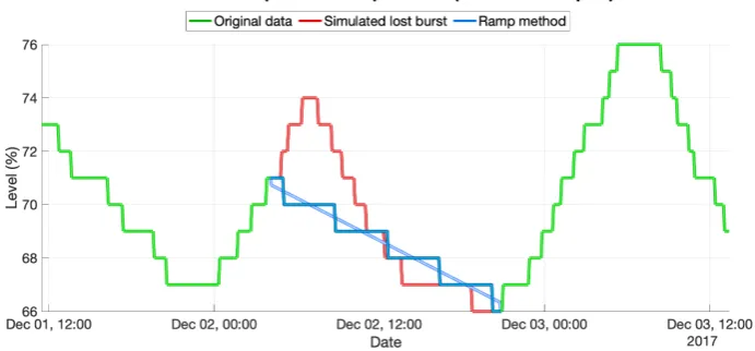
The tensor decompositions cannot work with empty data. One of the simplest strategies used with acceptable results in [14], called theramp methodis used in this study. Theramp methodconsists of filling the lost data by drawing a line between the last known sample before the lost burst starting,xn,
and the first known sample after the lost burst ending,xn+B+1, whereBis the length of the data burst
lost in number of samples. So that, considering a lost burst ofBsamples and the indexigoing from 1 toB, to use a constant increment (or decrement),m, and fill the entire lost burst,xn+imust be:
xn+i =xn+m·i for m= xn
−xn+B+1
B+1 . (1)
Fig.1shows the performance of theramp method.
Figure 1.First step of the data reconstruction method. The red line shows the burst of the simulated lost data. The blue line corresponds to the data reconstruction of the linear method called theramp method. The soft blue line shows the linear method result and the strong blue line shows the final signal reconstruction, which is adapted to the sensor resolution of 1%.
2.3. Burst centered tensorization
patterns on a daily and weekly scale. To take advantage of these regularities, a 3-dimensional tensor was composed. The first index indicates the 5-minute day-intervals fixed by the sample frequency of the SCADA system (so each day is represented by 288 samples). The second index indicates the day of the week (which is an index of 7 positions, corresponding to the days of the week). Finally, the third index depends on the number of weeks included in the tensornw. In this way, the 3-dimensional
tensor will have the following 288×7×nwstructure.
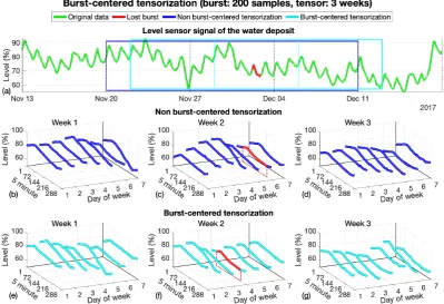
The proposed organization uses past and future data with respect to the burst location in order to contribute with past and future information. Typically, the way to organize the data into a tensor does not take into account the position of the lost data. In this work, aburst centered tensorization method is proposed, where the data selected to fill the tensor container depends on the burst location. Fig.2
shows this process. In Fig.2(a), the dark blue window shows the selection of data as was proposed in [14], in a typical way and with the data presented in a uni-dimensional view. The week where the burst is located is used as the central week, and some weeks before and some weeks after are taken, depending on the tensor sizenw. Note that to always have a central week in the tensornwthere
must be an odd value (3, 5, 7, ...). Through the dark blue window it can be seen how the burst is not exactly located in the center of the selected data, which would mean being in the center of the dark blue window, even if the week where the burst is located is selected as the central week. This happens because the burst is hardly located in the middle of a week, which only happens if the burst is located exactly in the center of Thursday. Theburst centered tensorizationforces the burst to be located in the center of the data selected. The cyan window in Fig.2(a) shows this new data selection, where the burst is placed exactly on the center of the window. Fig.2(b), (c) and (d) show thetensorizeddata by the typical way. The Fig.2(e), (f) and (g) show thetensorizeddata from theburst centered tensorization method, which placed the burst in the core of the tensor (in the center of the central day of the week, which is located in the middle of the tensor). As explained in [14], lost data bursts never exceed the day, meaning that their length,B, is always less than 288 samples and that the burst can be located in the center of a day. Thus, given aBburst in a tensorχI×J×K, the burst samples are placed at J= 4, K=0.5(W+1)with initial positionIi=0.5(288-B) according to and indexationχIi:Ii+B−1×4×0.5(W+1).
Note that the daily cycles of theburst centered tensorizationrarely start at 00:00 and the weeks do not start on Mondays, as occurred in [14], however there are always the same number of samples before and after the lost burst, which hardly happens with the previoustensorizationmethod.
2.4. Tucker and CP tensor decompositions overview
A tensor is a container that can arrange data inN-ways or dimensions. AnN-way tensor of real elements is denoted asχ∈RI1×I2×···×IN and its elements as:xi1,i2,...,iN. According this, anN×1 vector
xis considered a tensor of order one, and anN×MmatrixX(orXN×M), a tensor of order two. The procedure of reshaping a lower-dimensional original data (for instance a vector or a matrix) into a tensor is referred to astensorization. The process of reshaping tensors to vectors is named vectorization.
Low order tensor decompositions provide a simplified version of the data while making the relation between dimensions explicit. In the case of the 3-dimensional tensor χI×J×K the approximations are given in the form of a smaller tensor coreGL×M×N, (where I > L, J > M, andK>N) and theL,JandKeigenvectors of mode-1, -2, and -3 respectively which are organized as column vectors in matricesAI×L,BJ×M, andCK×N. The size (L,M,N) of the core determines the level of the decomposition.
There are many known tensor decompositions but overall of them the most widely used are the Tucker [15] and the CP [18] decompositions. In this work we only test those two. However, the method presented can be adapted to work with any one of them. These two are briefly presented below.
5 of 19
Figure 2.Example of the datatensorizationof a 3 week tensor with 200 samples of data burst lost. In figure a) the green line shows the original data and the red line shows the lost burst. The strong blue window shows the data introduced in thenon burst-centeredtensor and the soft blue one shows the data introduced inburst-centeredtensor, which forces the burst to be on the center of the window. Figures b), c), and d) show the three weeks of thenon burst-centeredtensor and the location of the burst, which is located on the central week but not on the center of this week. The figures e), f), and g) show the 3 weeks of theburst-centeredtensor and the new location of the burst in the core of the tensor, which is in the middle of the central week.
χI×J×K≈GL×M×N×1AI×L×2BJ×M×3CK×N, (2)
where the symbol×iis the n-way product of a tensor by a matrix; such a tensor operation defined,
for example, in [21].
The 3-way CANDECOMP/PARAFAC (from CANonical DECOMPosition/PARAllel FACtorization) model is commonly known as CP and can be seen as particular case of the Tucker decomposition when GD×D×D is diagonal. Taking this observation into account the CP decomposition can be written in the same terms as in the case of Tucker decomposition, as follows:
χI×J×K≈GD×D×D×1AI×D×2BJ×D×3CK×D (3)
although, beingGD×D×Ddiagonal, it is frequent to see it written in function of the elementsλiof
the diagonal such as:
χI×J×K≈
D
∑
i=1
λiai◦bi◦ci, (4)
where the symbol◦stands for the outer product and the column vectorsai,biandciare related
with the matrices of equ. (3) according to: AI×D = [a1· · ·aD], BJ×D = [b1· · ·bD] andCK×D =
[c1· · ·cD].
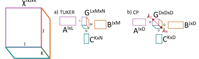
The algebra of tensors is explained in detail and often with the support of graphical illustrations in [10–12,20]. Fig.3shows a unified representation of both 3D tensor decompositions.
Figure 3.Diagram of theTensorizationmethods. a) Tucker model. b) CANDECOMP/PARAFAC (CP) model.
2.5. The continuity correction
This procedure was developed in order to maintain the continuity of the estimate provided by a tensor decomposition in its vector form ˆx and the known values of x at the edges of the burst. As consistently observed previously, the samples in the burst positions after a low-rank tensor reconstruction follow the original signal pretty well but with significant discontinuities in the extremes. Consideringx0to be the last original known sample before the burst and ˆx0the sample from the tensor
reconstruction in that position, we define the initial burst offset asO0=x0−xˆ0. Similarly, for a lost
burst of lengthB, the final burst offset can be defined as:OB+1= xB+1−xˆB+1. The corrected offset
estimates ˜xiare computed as follows:
˜
xi =xˆi+
(B−i)O0+ (i−1)OB+1
7 of 19
Figure 4.Second and third steps of the data reconstruction method. The green line is the original data, xi. The red line shows the 200 samples burst of simulated lost data. The Tucker decomposition (1,1,1) is used. The orange line is the result of the tensor process with this configuration, ˆxi. The blue arrows indicate the initial and the final offsets,O0andOB+1. The soft blue line show the effect of thecontinuity correction, ˜xiand the strong blue line shows the final signal reconstruction, which is adapted to the sensor resolution of 1%.
2.6. Signal smoothing
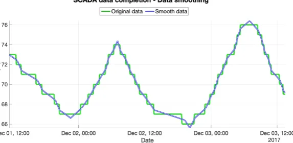
The tensor decomposition produces a continuous response. The sensor, however, measures the level as a percentage with resolution of 1%, providing a discrete signal of the deposit capacity. When the signal levels oscillate around the point of quantification, oscillations occur between adjacent discrete values. The goal of this section is to verify if a smoothing of the data applied before the tensor decomposition can help to improve the results.
The smoothing algorithm adopted isad hoc, developed considering the sensor way of working. The samples are processed in groups with the same integer value, and taking into account whether the signal is increasing, decreasing or is in a relative minimum or maximum. The blocks of samples of identical integer valueAare processed taking into account the values of the contiguous blocks. The procedure is effortless. There are more elaborate filtering methods but those introduce delays in the signal, and thus of that this straightforward solution has been chosen instead. If the block corresponds to a signal increment, a line with a positive slope is built with extreme valuesA-0.5 and A+0.5. If the block corresponds to a signal decrement, a line with a negative slope is built similarly. If it is detected that it is a local maximum or minimum, the block is replaced by a triangular shape with the corresponding orientation. Fig.5shows the smoothing performed through an example.
Figure 5.Smooth process applied to the level sensor signal before the second step of the methodology, thetensorizationof the data, to help on the tensor process to achieve a better estimation.
2.7. Double decomposition approach
In this section the proposed data completion method is presented through the sub-processes previously commented. As was already mentioned, only the two more widely known tensor decomposition models have been considered, these being the Tucker and the CP. Thus the configuration of both decomposition algorithms have been analyzed with the aim of taking the biggest advantage possible from each one.
In order to clarify the followed procedure, it is shown through a particular case in Figure6, where the steps of the process are represented by using a block diagram.
In that figure, vectorxis the input that contains the burst of missing values. The first step required is to choose the linear method of data completion that fills the data gap of the lost burst with a first simple first estimation. Theramp methodis the selected one, which draws a line to join the known extreme values that delimit the burst as explained in subsection2.2. It is a rough approximation, but does not need any configuration, which brings simplicity to the algorithm.
Once the data inxhas no empty values, and the positions of lost burst values have been saved, theburst centered tensorizationexplained in section2.3is applied. The tensor obtained isχ288×7×nw. To remember, its first dimension indexes the SCADA measurements taken in 24h every 5-minute, its second dimension indexes the 7 days to complete a week, and its third dimension indexes the numbernwof weeks considered (which is an odd number: 3 or 7 in the tests realized). In Figure.6the
particular case ofnw=7 is shown.
This is followed by the first tensor decomposition. The goal is to build a low-range approach of χ288×7×nw that is done by decomposing Tucker (4,6,1). The result is namedχ(2881)×7×nw. At that time, thecontinuity correctionis applied on the set of estimated samples which are in the position of the lost burst, with the aim to adapt the estimated signal fluctuation to the original data. That is, to use this set of samples to fill the same positions (those of the lost burst) in a new tensor, calledχ,288(1)times7×nw, which has the rest of positions filled with the original data. Note that bothχ288(1)×7×nwandχ,288(1)×7×nw have the same tensor arrangement, theburst centered tensorization.
The next step consists in doing the second tensor decomposition, now with the second core selected (Tucker(4,7,7) in the example) to obtain an approximation ofχ,288(1)×7×nw namedχ288(2)×7×nw. Again, the set of samples ofχ288(2)×7×nw located in the positions of the lost burst are taken to apply the continuity correctionwith the original data, and finally obtaining the SCADA data completion.
The Tucker(4,6,1) and Tucker(4,7,7) decomposition shown in Figure6(a) correspond to the values that optimize in our database the recovery of a burst of 200 lost samples when employing the tensorization of size 288×7×7 and the Tucker decomposition is used. The method is the same for the CP decomposition. The decomposition CP(1) and CP(15) shown in6(b) to optimize the recovery of a burst of 200 lost samples using thetensorizationof size 288×7×7 and the CP decomposition. The results are a statistical measure obtained after running 1000 simulations.
The study to determine the optimal size of these decompositions can be found later in subsection
3.1.2.
2.8. Algorithm performance evaluation
9 of 19
Figure 6.Graphic representation of thedouble decomposition methodfor both models checked, Tucker (a) and CP (b). In both cases the order of the decomposition shown is the optimized one in order to recover a burst of 200 lost samples when employing a tensor size of 288×7×7.
the nearest integer the values with decimals. Then, considering ˆxito be the samples provided by a
completion algorithm andxito be the true values that had been eliminated in the verified data set to
simulate a lost burst of lengthB, the MSE per sample is computed as:
MSE= 1
B
B
∑
i=1
q
(xi−xˆi)2 (6)
3. Results
In the first part of this section, the study conducted to find the orders of decomposition that optimize the MSE per sample is shown.
3.1. Optimal tensor decompositions
This exploration is performed by completing bursts of known length that have been randomly deleted from the reference database. A test of 1,000 simulations is done with 100 and 200 lost samples and using a 3 and a 7 weeks tensors. The results are given in terms of the MSE per sample, according to the exposed methodology.
The first test is done using only one decomposition and checking a set of different cores. This way the process stats are used to select the optimal core for the first decomposition, in terms of the MSE per sample. Then, to find the value of the second optimal decomposition core, the test is done with thedouble decompositionalgorithm. This time, the same sets of cores is checked on the second decomposition, using the optimal configuration found on the first test for the first decomposition. This exploration already allows us to see that the method is robust for small variants in the core used on the decomposition.
3.1.1. CP case
Here the results for the optimal CP decompositions configuration are presented when the length of the bursts are 100 and 200, and fortensorizations of 3 and 7 weeks of data. Four cases result from the combination of burst lengths and tensor sizes. Fig.7showsB = 100 with atensorization of (288×7×3); Fig.8, B = 100 with (288×7×7); Fig.9, B = 200 with (288×7×3); and Fig.10
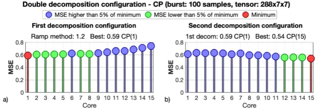
B=200 with (288×7×7). All these figures follow the same format. Figure a) shows, for different CP decomposition cores, the MSE per sample of the methodology with only one decomposition, applying thedata smoothing, theramp methodand theburst centered tensorization. Figure b) shows the MSE per sample obtained with thedouble decompositionmethodology, for different CP decomposition cores applied in the second stage, and using, as first decomposition core, the one which has given the lowest MSE value in the previous analysis. In both figures a) and b), the configuration that produces the minimum value is highlighted in red and the configurations that generate values very close to the minimum are highlighted in green .
Figure 7. Test of the double decomposition procedure configuration with the CP model for a 100 samples burst and the 3 weeks tensorχ288×7×3. (a) shows the MSE obtained applying only the first decomposition procedure, for different core configurations. (b) shows the MSE of thedouble decomposition methodfor different core configurations on the second decomposition, and using the best core configuration obtained on (a) for the first decomposition,G1×1×1. For each case the configuration with minimum MSE is marked in red and the configurations whose MSE rise with respect to the minimum is less than 5% are marked in green.
11 of 19
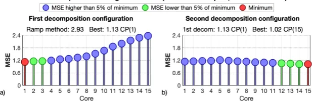
Figure 9. Test of thedouble decompositionprocedure configuration with the the CP model for a 200 samples burst and the 3 weeks tensorχ288×7×3. (a) shows the MSE obtained applying only the first decomposition procedure, for different core configurations. (b) shows the MSE of thedouble decomposition methodfor different core configurations on the second decomposition, and using the best core configuration obtained on (a) for the first decomposition,G1×1×1. For each case the configuration with minimum MSE is marked in red and the configurations whose MSE rise with respect to the minimum is less than 5% are marked in green.
Figure 10. Test of thedouble decompositionprocedure configuration with the CP model for a 200 samples burst and the 7 weeks tensorχ288×7×7. (a) shows the MSE obtained applying only the first decomposition procedure, for different core configurations. (b) shows the MSE of thedouble decomposition methodfor different core configurations on the second decomposition, and using the best core configuration obtained on (a) for the first decomposition,G1×1×1. For each case the configuration with minimum MSE is marked in red and the configurations whose MSE rise with respect to the minimum is less than 5% are marked in green.
As important aspects to emphasize, notice that in all the tested conditions of burst and tensor sizes, the best decomposition core for the first stage is the lowest one, CP(1). Then, using the CP(1) configuration on the first decomposition, in graph b), which shows the results for different core configurations on the second decomposition, it can be seen how the best option is to select the highest core configuration because, although in some cases it is not exactly the best, the MSE seems to have been stabilized. Therefore, for the CP method, the choice of the first decomposition core is very robust, and it has to be the lowest one. Then, for the second stage a higher decomposition core has to be selected , taking into account that there is a wide margin of acceptable configurations (values highlighted in green), because when the minimum is reached, the choice of an even higher decomposition core gives a very similar MSE.
3.1.2. Tucker case
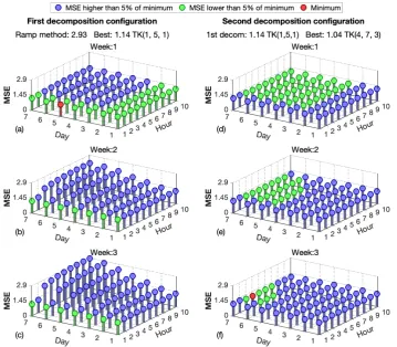
Determining the size of the two decompositions that minimize the MSE per sample, when using Tucker decomposition, is computationally expensive and difficult to visualize. This is because there are more parameters than in the CP model to configure the decomposition core. The number of parameters depends on the tensor structure, and in the proposed 3-dimensionstensorizationthis implies having three parameters.
The experiments carried out include the cases of the burst length 100 and 200 and thetensorizations χ288×7×3andχ288×7×7. Figures7and8deal with bursts of 100 missing samples andtensorizationsof χ288×7×3andχ288×7×7respectively. Figures9and10deal with bursts of 200 missing samples and tensorizationsofχ288×7×3andχ288×7×7.
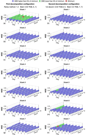
In this case, to see the optimization of Tuker model configuration graphically, one of the three parameters which have to be configured has been set, the one relative to the weeks number of data used. Then, using a matrix view, the MSE values of the combination of the other two can be further analyzed. For each figure, the first column of graphs represents the results corresponding to the first decomposition. The graphs of the second column show the MSE corresponding to the second decomposition after selecting the combination that gives the lowest value for the first one.
In all cases, the red dot represents the configuration with the lowest MSE value and the green points are those configurations with values very close to the minimum.
It is noted that the red dots are within the clusters of green points which represent quasi-optimal solutions. This means that there is a whole set of different solutions that behave in a very similar way to the optimal set. In general the best option is to select the minimum possible value on the parameter related to the number of weeks for the first decomposition and the maximum for the second one. The other two parameters seems to have more variability, but in general the parameter relative to the week day must be high, near the maximum, and the parameter relative to the day hour must be a little lower than it.
Some improvements for the method have been proposed, with the aim of refining it and obtaining better results. To see the effect of each of them the same 1,000 simulations are done without applying the improvements, followed by applying only one of them, applying some of them and finally applying them all together in Fig.15. The best results seem to be achieved with the rearrangement of the tensor using theburst centered tensorization, which is the best improvement if it is only applied to one of them on the methodology. Applying only the smooth process provides a little improvement on any case, not very high but constant for all the tensor and burst sizes checked.
A curious result of thedouble decompositionis that it seems to have, proportionally, a more positive effect when it is used in combination with the other options. This can be seen by comparing the MSE reduction obtained by applying only thedouble decompositioncompared to using a combination of smoothing andburst centered tensorizationor using all the improvements, specially with the Tucker model results.
With any size of tensor and burst the effect of each option is complementary to the others, which means that applying all of the improvements together provides a considerable positive impact in comparison to not using any of them in all the cases. Note that using different tensor sizes or to restoring bursts of different lengths results in a different optimal configuration of the decomposition core, although with similar characteristics, Fig. 7- Fig. 14. To show the robustness of the modified method which incorporates thedouble decomposition, the MSE obtained using different configurations for the first decomposition presented, specifically the ones found in the first column of Fig. 7- Fig.
13 of 19
Figure 11.Test of thedouble decompositionprocedure configuration with the Tucker model for a 100 samples burst and the 3 weeks tensorχ288×7×3. (a) shows the MSE obtained applying only the first decomposition procedure, for different core configurations. (b) shows the MSE of thedouble decomposition methodfor different core configurations on the second decomposition, and using the best core configuration obtained on (a) for the first decomposition,G6×3×1. For each case the configuration with minimum MSE is marked in red and the configurations whose MSE rise with respect to the minimum is less than 5% are marked in green.
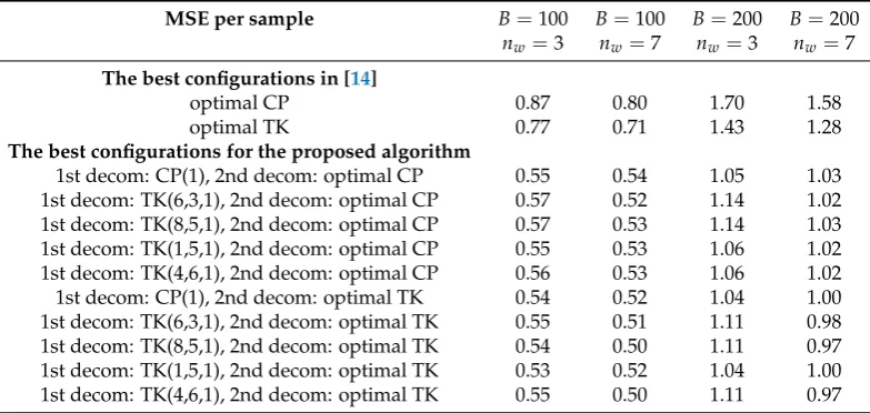
Table 1.MSE of the different tested methods. The results of 100 and 200 lost samples,B, are shown working with a 3 and 7 weeks of tensor size,nw. "The best configurations in [14]" show the minimum MSE obtained for the algorithm presented in [14], with the CP and the Tucker models. "The best configurations for the proposed algorithm" show the minimum MSE obtained for different pairs of decompositions. In these cases, only the core of the first decomposition is fixed, and it is shown the minimum MSE obtained with the best core for the second decomposition.
MSE per sample B=100 B=100 B=200 B=200
nw=3 nw=7 nw=3 nw=7
The best configurations in [14]
optimal CP 0.87 0.80 1.70 1.58
optimal TK 0.77 0.71 1.43 1.28
The best configurations for the proposed algorithm
15 of 19
Figure 13.Test of thedouble decompositionprocedure configuration with the Tucker model for a 100 samples burst and the 7 weeks tensorχ288×7×7. (a) shows the MSE obtained applying only the first decomposition procedure, for different core configurations. (b) shows the MSE of thedouble decomposition methodfor different core configurations on the second decomposition, and using the best core configuration obtained on (a) for the first decomposition,G8×5×1. For each case the configuration with minimum MSE is marked in red and the configurations whose MSE rise with respect to the minimum is less than 5% are marked in green.
17 of 19
Figure 15.MSE of the proposed improvements. All of them are tested with 100 and 200 samples of data burst lost and with 3 and 7 weeks oftensorizeddata. The orange line indicates the best result obtained in [14]. TheSmoothis the result of applying only the smooth process to the signal beforetensorizing it. Theburst centered tensorizationis the result of the rearrangement of the tensor according the burst location. TheDouble decomis the result of applying the decomposition two times, withG4×6×1and G4×7×7for Tuker, andG1×1×1andG15×15×15for CP. TheDS-Bcis the result of combining the data smoothing and theburst centered tensorizationwithout using the double decomposition. TheAll with CP and theAll with TKare the results of applying all the proposed algorithm with the CP and the Tucker models respectively.
Figure 16.Example of the reconstruction methodology with double decomposition. The green line shows the original data and the red line the burst of lost samples. The orange line is the linear estimation with theramp method. The purple line is the result of the firsttensorizationprocedure with Tuker using G4×6×1. The blue line shows the result of the secondtensorizationprocedure withG4×7×7.
4. Conclusions
Completing data lost in bursts remains a difficult challenge and is where most data completion methods fail. However, data being lost in bursts is quite common. It is often associated with the failure of a component involved in capturing or transmitting the data. In the contribution of [14] it is presented anad hocdata completion method is presented to recover data lost in bursts that outperforms the methods available in the literature for the proposed application. This work improves the method in [14], which is taken as a reference for the new algorithm evaluation and for comparison purposes. It is also often difficult to evaluate data completion methods. In this article, intensive experiments on a verified database were carried out by erasing data statistically and comparing the results of the algorithms with the original data are carried out. The method incorporates fundamental novelties such as a newtensorizationmethod, theburst centered tensorization, and the application of two tensor decomposition, one after the other.
Note that the MSE corresponding to a 100 samples burst falls from 0.71, the best result obtained in [14], to 0.50, the best result obtained with this new methodology. Thus, approximately a 39.5% of reduction is achieved. In the case of a 200 samples burst the MSE falls from 1.28 to 0.97 which is approximately a 24.2% of reduction.
A signal reconstruction example of this procedure is shown in Fig.16usingG4×6×1andG4×7×7, the best core configurations for the double decomposition according to the tests for the Tucker model in the case of a 200 samples of burst length.
Author Contributions:conceptualization, P.M.-P.and A.M.-S.; methodology, P.M.-P., M.S.-S. and A.M.-S; software, P.M.-P. and A.M.-S. ; validation, P.M.-P., M.S.-S and A.M.-S.; formal analysis, P.M.-P., M.S.-S and A.M.-S; investigation, P.M.-P. and A.M.-S.; resources, P.M.-P. and M.S.-S; writing–original draft preparation, P.M.-P. and A.M.-S.; writing–review and editing, P.M.-P. and A.M.-S.; supervision, P.M.-P. and M.S.-S.; funding acquisition, P.M.-P. and M.S.-S.
Funding:Financial support by the Agency for Management of University and Research Grants (AGAUR) of the Catalan Government to Arnau Martí-Sarri is gratefully acknowledged.
Acknowledgments:We thank the company Aigües de Vic S.A. for giving us access to their databases to perform this research.
Conflicts of Interest:The authors declare no conflict of interest.
References
1. Langhammer, J.; ˇCesák, J. Applicability of a Nu-Support Vector Regression Model for the Completion of Missing Data in Hydrological Time Series.Water2016,8. doi:10.3390/w8120560.
2. Ahlheim, M.; Frör, O.; Luo, J.; Pelz, S.; Jiang, T. Towards a Comprehensive Valuation of Water Management Projects When Data Availability Is Incomplete — The Use of Benefit Transfer Techniques. Water2015, 7, 2472–2493. doi:10.3390/w7052472.
3. Zhao, Q.; Zhu, Y.; Wan, D.; Yu, Y.; Cheng, X. Research on the Data-Driven Quality Control Method of Hydrological Time Series Data. Water2018,10. doi:10.3390/w10121712.
4. Ekeu-wei, I.T.; Blackburn, G.A.; Pedruco, P. Infilling Missing Data in Hydrology: Solutions Using Satellite Radar Altimetry and Multiple Imputation for Data-Sparse Regions.Water2018,10. doi:10.3390/w10101483. 5. Blanch, J.; Puig, V.; Saludes, J.; Quevedo, J. Arima models for data consistency of flowmeters in water
distribution networks. IFAC Proceedings Volumes2009,42, 480–485.
6. Lamrini, B.; Lakhal, E.K.; Le Lann, M.V.; Wehenkel, L. Data validation and missing data reconstruction using self-organizing map for water treatment. Neural Computing and Applications2011,20, 575–588. 7. Puig, V.; Ocampo-Martinez, C.; Pérez, R.; Cembrano, G.; Quevedo, J.; Escobet, T.Real-Time Monitoring and
Operational Control of Drinking-Water Systems; Springer, 2017.
8. Acar, E.; Dunlavy, D.M.; Kolda, T.G.; Mørup, M. Scalable tensor factorizations for incomplete data. Chemometrics and Intelligent Laboratory Systems2011,106, 41–56.
19 of 19
10. Mørup, M. Applications of tensor (multiway array) factorizations and decompositions in data mining. Wiley Interdisciplinary Reviews: Data Mining and Knowledge Discovery2011,1, 24–40.
11. Kolda, T.G.; Bader, B.W. Tensor decompositions and applications.SIAM review2009,51, 455–500. 12. Cichocki, A.; Mandic, D.; De Lathauwer, L.; Zhou, G.; Zhao, Q.; Caiafa, C.; Phan, H.A. Tensor
decompositions for signal processing applications: From two-way to multiway component analysis. IEEE Signal Processing Magazine2015,32, 145–163.
13. Comon, P. Tensors: a brief introduction. IEEE Signal Processing Magazine2014,31, 44–53.
14. Marti-Puig, P.; Martí-Sarri, A.; Serra-Serra, M. Different Approaches to SCADA Data Completion in Water Networks. Water2019,11, 1023.
15. Tucker, L.R. Some mathematical notes on three-mode factor analysis. Psychometrika1966,31, 279–311. 16. Carroll, J.D.; Chang, J.J. Analysis of individual differences in multidimensional scaling via an N-way
generalization of “Eckart-Young” decomposition. Psychometrika1970,35, 283–319.
17. De Lathauwer, L.; De Moor, B.; Vandewalle, J. A multilinear singular value decomposition. SIAM journal on Matrix Analysis and Applications2000,21, 1253–1278.
18. Harshman, R.A. Foundations of the PARAFAC procedure: Models and conditions for an" explanatory" multimodal factor analysis.Working Papers in Phonetics1970,UCLA Working Papers in Phonetics, 16, 1–84. 19. Sørensen, M.; Lathauwer, L.D.; Comon, P.; Icart, S.; Deneire, L. Canonical polyadic decomposition
with a columnwise orthonormal factor matrix. SIAM Journal on Matrix Analysis and Applications2012, 33, 1190–1213.
20. Sidiropoulos, N.D.; De Lathauwer, L.; Fu, X.; Huang, K.; Papalexakis, E.E.; Faloutsos, C. Tensor decomposition for signal processing and machine learning. IEEE Transactions on Signal Processing2017, 65, 3551–3582.
21. Kolda, T.G. Multilinear operators for higher-order decompositions. Technical report, Sandia National Laboratories, 2006.