Implementing Gentry’s Fully-Homomorphic Encryption Scheme
Craig Gentry Shai Halevi
IBM Research February 4, 2011
Abstract
We describe a working implementation of a variant of Gentry’s fully homomorphic encryption scheme (STOC 2009), similar to the variant used in an earlier implementation effort by Smart and Vercauteren (PKC 2010). Smart and Vercauteren implemented the underlying “somewhat homomorphic” scheme, but were not able to implement the bootstrapping functionality that is needed to get the complete scheme to work. We show a number of optimizations that allow us to implement all aspects of the scheme, including the bootstrapping functionality.
Our main optimization is a key-generation method for the underlying somewhat homomor-phic encryption, that does not require full polynomial inversion. This reduces the asymptotic complexity from ˜O(n2.5) to ˜O(n1.5) when working with dimension-n lattices (and practically
reducing the time from many hours/days to a few seconds/minutes). Other optimizations in-clude a batching technique for encryption, a careful analysis of the degree of the decryption polynomial, and some space/time trade-offs for the fully-homomorphic scheme.
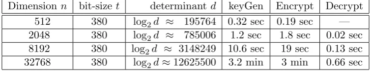
We tested our implementation with lattices of several dimensions, corresponding to several security levels. From a “toy” setting in dimension 512, to “small,” “medium,” and “large” settings in dimensions 2048, 8192, and 32768, respectively. The public-key size ranges in size from 70 Megabytes for the “small” setting to 2.3 Gigabytes for the “large” setting. The time to run one bootstrapping operation (on a 1-CPU 64-bit machine with large memory) ranges from 30 seconds for the “small” setting to 30 minutes for the “large” setting.
1
Introduction
Encryption schemes that support operations on encrypted data (aka homomorphic encryption) have a very wide range of applications in cryptography. This concept was introduced by Rivest et al. shortly after the discovery of public key cryptography [14], and many known public-key cryptosystems support either addition or multiplication of encrypted data. However, supporting both at the same time seems harder, and until very recently all the attempts at constructing so-called “fully homomorphic” encryption turned out to be insecure.
Toward a bootstrappable scheme, Gentry described in [4] a somewhat homomorphic scheme, which is roughly a GGH-type scheme [8, 10] over ideal lattices. Gentry later proved [5] that with an appropriate key-generation procedure, the security of that scheme can be (quantumly) reduced to the worst-case hardness of some lattice problems in ideal lattices.
This somewhat homomorphic scheme is not yet bootstrappable, so Gentry described in [4] a transformation to squash the decryption procedure, reducing the degree of the decryption poly-nomial. This is done by adding to the public key an additional hint about the secret key, in the form of a “sparse subset-sum” problem (SSSP). Namely the public key is augmented with a big set of vectors, such that there exists a very sparse subset of them that adds up to the secret key. A ciphertext of the underlying scheme can be “post-processed” using this additional hint, and the post-processed ciphertext can be decrypted with a low-degree polynomial, thus obtaining a bootstrappable scheme.
Stehl´e and Steinfeld described in [18] two optimizations to Gentry’s scheme, one that reduces the number of vectors in the SSSP instance, and another that can be used to reduce the degree of the decryption polynomial (at the expense of introducing a small probability of decryption errors). We mention that in our implementation we use the first optimization but not the second.1 Some improvements to Gentry’s key-generation procedure were discussed in [11].
1.1 The Smart-Vercauteren implementation
The first attempt to implement Gentry’s scheme was made in 2010 by Smart and Vercauteren [17]. They chose to implement a variant of the scheme using “principal-ideal lattices” of prime determinant. Such lattices can be represented implicitly by just two integers (regardless of their dimension), and moreover Smart and Vercauteren described a decryption method where the secret key is represented by a single integer. Smart and Vercauteren were able to implement the underlying somewhat homomorphic scheme, but they were not able to support large enough parameters to make Gentry’s squashing technique go through. As a result they could not obtain a bootstrappable scheme or a fully homomorphic scheme.
One obstacle in the Smart-Vercauteren implementation was the complexity of key generation for the somewhat homomorphic scheme: For one thing, they must generate very many candidates before they find one whose determinant is prime. (One may need to try as many asn1.5candidates when working with lattices in dimension n.) And even after finding one, the complexity of com-puting the secret key that corresponds to this lattice is at least ˜Θ(n2.5) for lattices in dimensionn. For both of these reasons, they were not able to generate keys in dimensionsn >2048.
Moreover, Smart and Vercauteren estimated that the squashed decryption polynomial will have degree of a few hundreds, and that to support this procedure with their parameters they need to use lattices of dimension at leastn= 227(≈1.3×10⁸), which is well beyond the capabilities of the key-generation procedure.
1.2 Our implementation
We continue in the same direction of the Smart-Vercauteren implementation and describe opti-mizations that allow us to implement also the squashing part, thereby obtaining a bootstrappable scheme and a fully homomorphic scheme.
For key-generation, we present a new faster algorithm for computing the secret key, and also eliminate the requirement that the determinant of the lattice be prime. We also present many
sim-1The reason we do not use the second optimization is that the decryption error probability is too high for our
plifications and optimizations for the squashed decryption procedure, and as a result our decryption polynomial has degree only fifteen. Finally, our choice of parameters is somewhat more aggressive than Smart and Vercauteren (which we complement by analyzing the complexity of known attacks). Differently from [17], we decouple the dimension nfrom the size of the integers that we choose during key generation.2 Decoupling these two parameters lets us decouple functionality from se-curity. Namely, we can obtain bootstrappable schemes in any given dimension, but of course the schemes in low dimensions will not be secure. Our (rather crude) analysis suggests that the scheme may be practically secure at dimensionn= 213 orn= 215, and we put this analysis to the test by publishing a few challenges in dimensions from 512 up to 215.
1.3 Organization
We give some background in Section 2, and then the report is organized in two parts. In Part I we describe our implementation of the underlying “somewhat homomorphic” encryption scheme, and in Part II we describe our optimizations that are specific to the bootstrapping functionality. To aid reading, we list here all the optimizations that are described in this report, with pointers to the sections where they are presented.
Somewhat-homomorphic scheme.
1. We replace the Smart-Vercauteren requirement [17] that the lattice has prime determinant, by the much weaker requirement that the Hermite normal form (HNF) of the lattice has a particular form, as explained in Step 3 of Section 3. We also provide a simple criterion for checking for this special form.
2. We decrypt using a single coefficient of the secret inverse polynomial (similarly to Smart-Vercauteren [17]), but for convenience we use modular arithmetic rather than rational division. See Section 6.1.
3. We use a highly optimized algorithm for computing the resultant and one coefficient of the inverse of a given polynomialv(x) with respect tof(x) =x2m±1 (without having to compute the entire inverse). This is probably the most algorithmically interesting part of this work. See Section 4.
4. We use batch techniques to speed-up encryption. Specifically, we use an efficient algorithm for batch evaluation of many polynomials with small coefficients on the same point. See Section 5. Our algorithm, when specialized to evaluating a single polynomial, is essentially the same as Avanzi’s trick [1], which itself is similar to the algorithm of Paterson and Stockmeyer [12]. The time to evaluatekpolynomials is onlyO(√k) more than evaluating a single polynomial.
Fully homomorphic scheme.
5. The secret key in our implementation is a binary vector of lengthS≈1000, with onlys= 15 bits set to one, and the others set to zero. We get significant speedup by representing the secret key in s groups of S bits each, such that each group has a single 1-bit in it. See Section 8.1.
6. The public key of the bootstrappable scheme contains an instance of the sparse-subset-sum problem, and we use instances that have a very space-efficient representation. Specifically, we derive our instances from geometric progressions. See Section 9.1.
7. Similarly, the public key of the fully homomorphic scheme contains an encryption of all the secret-key bits, and we use a space-time tradeoff to optimize the space that it takes to store all these ciphertexts without paying too much in running time. See Section 9.2.
Finally, our choice of parameters is presented in Section 10, and some performance numbers are given in Section 11. Throughout the text we put more emphasis on concrete parameters than on asymptotics, asymptotic bounds can be found in [18].
2
Background
Notations. Throughout this report we use ‘·’ to denote scalar multiplication and ‘×’ to denote
any other type of multiplication. For integersz, d, we denote the reduction ofzmodulodby either [z]d or ⟨z⟩d. We use [z]d when the operation maps integers to the interval [−d/2, d/2), and use
⟨z⟩d when the operation maps integers to the interval [0, d). We use the generic “zmodd” when the specific interval does not matter (e.g., mod 2). For example we have [13]5 =−2 vs. ⟨13⟩5 = 3, but [9]7 =⟨9⟩7 = 2.
For a rational number q, we denote by⌈q⌋ the rounding ofq to the nearest integer, and by [q] we denote the distance between q and the nearest integer. That is, if q = ab then [q] def= [a]b
b and
⌈q⌋ def= q −[q]. For example, ⌈135⌋ = 3 and [135] = −52. These notations are extended to vectors in the natural way: for example if⃗q =⟨q0, q1, . . . , qn−1⟩ is a rational vector then rounding is done coordinate-wise, ⌈⃗q⌋=⟨⌈q0⌋,⌈q1⌋, . . . ,⌈qn−1⌋⟩.
2.1 Lattices
A full-rankn-dimensional latticeis a discrete subgroup of Rn, concretely represented as the set of all integer linear combinations of somebasis B = (⃗b1, . . . ,⃗bn)∈Rn of linearly independent vectors. Viewing the vectors⃗bi as the rows of a matrixB ∈Rn×n, we have:
L=L(B) ={⃗y×B : ⃗y∈Zn}.
Every lattice (of dimension n > 1) has an infinite number of lattice bases. IfB1 and B2 are two lattice bases of L, then there is some unimodular matrix U (i.e., U has integer entries and det(U) =±1) satisfying B1 =U ×B2. Since U is unimodular, |det(Bi)|is invariant for different bases of L, and we may refer to it as det(L). This value is precisely the size of the quotient group
Zn/L if L is an integer lattice. To basis B of lattice L we associate the half-open parallelepiped
P(B)← {∑ni=1xi⃗bi :xi ∈[−1/2,1/2)}. The volume of P(B) is precisely det(L).
For⃗c∈Rn and basisB of L, we use⃗cmodB to denote the unique vector⃗c′ ∈ P(B) such that
⃗c−c⃗′ ∈L. Given⃗candB,⃗cmodB can be computed efficiently as⃗c−⌊⃗c×B−1⌉×B = [⃗c×B−1]×B. (Recall that⌊·⌉ means rounding to the nearest integer and [·] is the fractional part.)
Every full-rank lattice has a unique Hermite normal form (HNF) basis where bi,j = 0 for all
i < j (lower-triangular),bj,j >0 for allj, and for alli > j bi,j ∈[−bj,j/2,+bj,j/2). Given any basis
Short vectors and Bounded Distance Decoding. The length of the shortest nonzero vector in a latticeL is denotedλ1(L), and Minkowski’s theorem says that for anyn-dimensional latticeL (n > 1) we haveλ1(L)<√n·det(L)1/n. Heuristically, for random lattices the quantity det(L)1/n serves as a threshold: fort≪det(L)1/n we don’t expect to find any nonzero vectors inLof size t, but fort≫det(L)1/n we expect to find exponentially many vectors inL of size t.
In the “bounded distance decoding” problem (BDDP), one is given a basisB of some latticeL, and a vector⃗c that is very close to some lattice point of L, and the goal is to find the point in L
nearest to⃗c. In the promise problem γ-BDDP, we have a parameter γ >1 and the promise that dist(L, ⃗c) def= min⃗v∈L{∥⃗c−⃗v∥} ≤ det(L)1/n/γ. (BDDP is often defined with respect to λ1 rather than with respect to det(L)1/n, but the current definition is more convenient in our case.)
Gama and Nguyen conducted extensive experiments with lattices in dimensions 100-400 [3], and concluded that for those dimensions it is feasible to solve γ-BDDP when γ > 1.01n ≈ 2n/70. More generally, the best algorithms for solving the γ-BDDP in n-dimensional lattices take time exponential inn/logγ. Specifically, currently known algorithms can solve dimension-n γ-BDDP in time 2kup toγ = 2
µn
k/logk, whereµis a parameter that depends on the exact details of the algorithm.
(Extrapolating from the Gama-Nguyen experiments, we expect something likeµ∈[0.1,0.2].)
2.2 Ideal lattices
Letf(x) be an integer monic irreducible polynomial of degreen. In this paper, we usef(x) =xn+1, wheren is a power of 2. LetR be the ring of integer polynomials modulo f(x),Rdef= Z[x]/(f(x)). Each element of R is a polynomial of degree at most n−1, and thus is associated to a coefficient vector in Zn. This way, we can view each element of R as being both a polynomial and a vector. For ⃗v(x), we let ∥⃗v∥ be the Euclidean norm of its coefficient vector. For every ring R, there is an associated expansion factor γMult(R) such that ∥⃗u×⃗v∥ ≤γMult(R)· ∥⃗u∥ · ∥⃗v∥, where ×denotes multiplication in the ring. When f(x) =xn+ 1, γMult(R) is
√
n. However, for “random vectors”
⃗
u, ⃗v the expansion factor is typically much smaller, and our experiments suggest that we typically have ∥⃗u×⃗v∥ ≈ ∥⃗u∥ · ∥⃗v∥.
Let I be an ideal ofR – that is, a subset of R that is closed under addition and multiplication by elements of R. Since I is additively closed, the coefficient vectors associated to elements of I
form alattice. We callI anideal latticeto emphasize this object’s dual nature as an algebraic ideal and a lattice.3Ideals have additive structure as lattices, but they also have multiplicative structure. The product IJ of two ideals I and J is the additive closure of the set {⃗v×w⃗ : ⃗v ∈ I, ⃗w ∈ J}, where ‘×’ is ring multiplication. To simplify things, we will use principal ideals of R – i.e., ideals with a single generator. The ideal (⃗v) generated by⃗v∈R corresponds to the lattice generated by
the vectors{⃗vi def
= ⃗v×xi modf(x) :i∈[0, n−1]}; we call this therotation basisof the ideal lattice (⃗v).
Let K be a field containing the ringR (in our case K =Q[x]/(f(x))). Theinverse of an ideal
I ⊆R isI−1={w⃗ ∈K:∀⃗v∈I, ⃗v×w⃗ ∈R}. The inverse of a principal ideal (⃗v) is given by (⃗v−1), where the inverse⃗v−1 is taken in the fieldK.
2.3 GGH-type cryptosystems
We briefly recall Micciancio’s “cleaned-up version” of GGH cryptosystems [8, 10]. The secret and public keys are “good” and “bad” bases of some lattice L. More specifically, the key-holder
3
generates a good basis by choosingBsk to be a basis of short, “nearly orthogonal” vectors. Then it sets the public key to be the Hermite normal form of the same lattice,Bpk
def
= HNF(L(Bsk)). A ciphertext in a GGH-type cryptosystem is a vector ⃗c close to the lattice L(Bpk), and the message which is encrypted in this ciphertext is somehow embedded in the distance from⃗c to the nearest lattice vector. To encrypt a message m, the sender chooses a short “error vector” ⃗e that encodes m, and then computes the ciphertext as⃗c ← ⃗emodBpk. Note that if⃗e is short enough (i.e., less than λ1(L)/2), then it is indeed the distance between⃗cand the nearest lattice point.
To decrypt, the key-holder uses its “good” basis Bsk to recover⃗e by setting ⃗e ← ⃗cmodBsk, and then recovers m from ⃗e. The reason decryption works is that, if the parameters are chosen correctly, then the parallelepiped P(Bsk) of the secret key will be a “plump” parallelepiped that contains a sphere of radius bigger than ∥⃗e∥, so that ⃗e is the point inside P(Bsk) that equals ⃗c modulo L. On the other hand, the parallelepiped P(Bpk) of the public key will be very skewed, and will not contain a sphere of large radius, making it useless for solving BDDP.
2.4 Gentry’s somewhat-homomorphic cryptosystem
Gentry’s somewhat homomorphic encryption scheme [4] can be seen as a GGH-type scheme over ideal lattices. The public key consists of a “bad” basisBpk of an ideal lattice J, along with some basisBIof a “small” idealI (which is used to embed messages into the error vectors). For example, the small idealI can be taken to beI = (2), the set of vectors with all even coefficients.
A ciphertext in Gentry’s scheme is a vector close to aJ-point, with the message being embedded in the distance to the nearest lattice point. More specifically, the plaintext space is {0,1}, which is embedded inR/I ={0,1}n by encoding 0 as 0nand 1 as 0n−11. For an encoded bitm⃗ ∈ {0,1}n we set⃗e= 2⃗r+m⃗ for a random small vector⃗r, and then output the ciphertext⃗c←⃗emodBpk.
The secret key in Gentry’s scheme (that plays the role of the “good basis” of J) is just a short vectorw⃗ ∈J−1. Decryption involves computing the fractional part [w⃗×⃗c]. Since⃗c=⃗j+⃗efor some
j∈J, then w⃗×⃗c=w⃗×⃗j+w⃗×e⃗. Butw⃗×⃗j is inRand thus an integer vector, sow⃗×⃗candw⃗×⃗e
have the same fractional part, [w⃗ ×⃗c] = [w⃗ ×⃗e]. Ifw⃗ and⃗eare short enough – in particular, if we have the guarantee that all of the coefficients ofw⃗×⃗ehave magnitude less than 1/2 – then [w⃗×⃗e] equalsw⃗×⃗eexactly. Fromw⃗×⃗e, the decryptor can multiply byw⃗−1 to recover⃗e, and then recover
⃗
m←⃗emod 2. The actual decryption procedure from [4] is slightly different, however. Specifically,
⃗
w is “tweaked” so that decryption can be implemented asm⃗ ←⃗c−[w⃗ ×⃗c] mod 2 (when I = (2)). The reason that this scheme is somewhat homomorphic is that for two ciphertexts⃗c1 =⃗j1+⃗e1 and⃗c2 =⃗j2+⃗e2, their sum is⃗j3+⃗e3 where⃗j3 =⃗j1+⃗j2 ∈J and ⃗e3 =⃗e1+⃗e2 is small. Similarly, their product is⃗j4+⃗e4 where⃗j4 =⃗j1×(⃗j2+⃗e2) +⃗e1×⃗j2 ∈J and e⃗4 =⃗e1×⃗e2 is still small. If fresh encrypted ciphertexts are very very close to the lattice, then it is possible to add and multiply ciphertexts for a while before the error grows beyond the decryption radius of the secret key.
2.4.1 The Smart-Vercauteren Variant
Smart and Vercauteren [17] work over the ring R =Z[x]/fn(x), where fn(x) = xn+ 1 and n is a power of two. The idealJ is set as a principal ideal by choosing a vector⃗v at random from some
n-dimensional cube, subject to the condition that the determinant of (⃗v) is prime, and then setting
ideal lattice is
HNF(J) =
d 0 0 0 0
−r 1 0 0 0
−[r2]
d 0 1 0 0
−[r3]d 0 0 1 0 . ..
−[rn−1]d 0 0 0 1
(1)
It is easy to see that reducing a vector⃗amodulo HNF(J) consists of evaluating the associated poly-nomiala(x) at the pointrmodulod, then outputting the vector⟨[a(r)]d,0,0, . . . ,0⟩(see Section 5). Hence encryption of a vector ⟨m,0,0, . . . ,0⟩ with m ∈ {0,1} can be done by choosing a random small polynomialu(x) and evaluating it at r, then outputting the integerc←[2u(r) +m]d.
Smart and Vercauteren also describe a decryption procedure that uses a single integerw as the secret key, settingm←(c−⌈cw/d⌋) mod 2. Jumping ahead, we note that our decryption procedure from Section 6 is very similar, except that for convenience we replace the rational divisioncw/dby modular multiplication [cw]d.
2.5 Gentry’s fully-homomorphic scheme
As explained above, Gentry’s somewhat-homomorphic scheme can evaluate low-degree polynomials but not more. Once the degree (or the number of terms) is too large, the error vector⃗egrows beyond the decryption capability of the private key. Gentry solved this problem using bootstrapping. He observed in [4] that a scheme that can homomorphically evaluate its own decryption circuit plus one additional operation, can be transformed into a fully-homomorphic encryption. In more details, fix two ciphertexts⃗c1, ⃗c2 and consider the functions
DAdd⃗c1,⃗c2(sk) def
= Decsk(⃗c1) +Decsk(⃗c2) and DMul⃗c1,⃗c2(sk) def
= Decsk(⃗c1)×Decsk(⃗c2).
A somewhat-homomorphic scheme is called “bootstrappable” if it is capable of homomorphically evaluating the functionsDAdd⃗c1,⃗c2 andDMul⃗c1,⃗c2 for any two ciphertexts⃗c1, ⃗c2. Given a bootstrap-pable scheme that is also circular secure, it can be transformed into a fully-homomorphic scheme by adding to the public key an encryption of the secret key, c⃗∗ ← Encpk(sk). Then given any two ciphertexts c⃗1, c⃗2, the addition/multiplication of these two ciphertexts can be computed by homomorphically evaluating the functionsDAdd⃗c1,⃗c2(c⃗∗) or DMul⃗c1,⃗c2(c⃗∗). Note that the error does not grow, since we always evaluate these functions on the fresh ciphertext c⃗∗ from the public key.
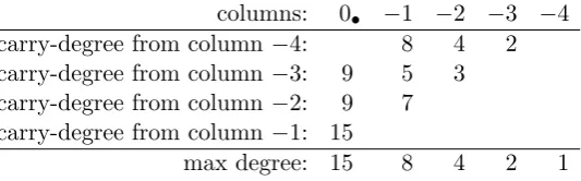
Unfortunately, the somewhat-homomorphic scheme from above is not bootstrappable. Although it is capable of evaluating low-degree polynomials, the degree of its decryption function, when expressed as a polynomial in the secret key bits, is too high. To overcome this problem Gentry shows how to “squash the decryption circuit”, transforming the original somewhat-homomorphic scheme E into a scheme E∗ that can correctly evaluate any circuit that E can, but where the complexity ofE∗’s decryption circuit is much less thanE’s. In the original somewhat-homomorphic schemeE, the secret key is a vectorw⃗. In the new schemeE∗, the public key includes an additional “hint” about w⃗ – namely, a big set of vectorsS ={⃗xi :i= 1,2, . . . , S} that have a hidden sparse subsetT that adds up tow⃗. The secret key ofE∗is the characteristic vector of the sparse subsetT, which is denoted⃗σ =⟨σ1, σ2, . . . , σS⟩.
as a polynomial in the σi’s of degree roughly the size of the sparse subset T. (The underlying algorithm could be a simple grade-school addition – add up the least significant column, bring a carry bit over to the next column if necessary, and so on.) With appropriate setting of the parameters, the subset T can be made small enough to get a bootstrappable scheme.
Part I
The “Somewhat Homomorphic” Scheme
3
Key generation
We adopt the Smart-Vercauteren approach [17], in that we also use principal-ideal lattices in the
ring of polynomials modulo fn(x) def= xn+ 1 with na power of two. We do not require that these principal-ideal lattices have prime determinant, instead we only need the Hermite normal form to have the same form as in Equation (1). During key-generation we choose ⃗v at random in some cube, verify that the HNF has the right form, and work with the principal ideal (⃗v). We have two parameters: the dimensionn, which must be a power of two, and the bit-sizetof coefficients in the generating polynomial. Key-generation consists of the following steps:
1. Choose a random n-dimensional integer lattice ⃗v, where each entry vi is chosen at random as a t-bit (signed) integer. With this vector ⃗v we associate the formal polynomial v(x) def=
∑n−1
i=0 vixi, as well as the rotation basis:
V =
v0 v1 v2 vn−1
−vn−1 v0 v1 vn−2
−vn−2 −vn−1 v0 vn−3 . ..
−v1 −v2 −v3 v0
(2)
Thei’th row is a cyclic shift of⃗vbyipositions to the right, with the “overflow entries” negated. Note that the i’th row corresponds to the coefficients of the polynomial vi(x) = v(x)×xi (modfn(x)). Note that just like V itself, the entire lattice L(V) is also closed under “rota-tion”: Namely, for any vector⟨u0, u1, . . . , un−1⟩ ∈ L(V), also the vector⟨−un−1, u0, . . . , un−2⟩ is inL(V).
2. Next we compute the scaled inverse ofv(x) modulofn(x), namely an integer polynomialw(x) of degree at most n−1, such that
w(x)×v(x) =constant (modfn(x)).
Specifically, this constant is the determinant of the lattice L(V), which must be equal to the resultant of the polynomials v(x) and fn(x) (since fn is monic). Below we denote the resultant byd, and denote the coefficient-vector ofw(x) byw⃗ =⟨w0, w1, . . . , wn−1⟩. It is easy to check that the matrix
W =
w0 w1 w2 wn−1
−wn−1 w0 w1 wn−2
−wn−2 −wn−1 w0 wn−3 . ..
−w1 −w2 −w3 w0
is the scaled inverse ofV, namelyW×V =V×W =d·I. One way to compute the polynomial
w(x) is by applying the extended Euclidean-GCD algorithm (for polynomials) to v(x) and
fn(x). See Section 4 for a more efficient method of computingw(x).
3. We also check that this is a good generating polynomial. We consider ⃗v to be good if the Hermite-Normal-form of V has the same form as in Equation (1), namely all except the leftmost column equal to the identity matrix. See below for a simple check that the⃗vis good, in our implementation we test this condition while computing the inverse.
It was observed by Nigel Smart that the HNF has the correct form whenever the determinant is odd and square-free. Indeed, in our tests this condition was met with probability roughly 0.5, irrespective of the dimension and bit length, with the failure cases usually due to the determinant ofV being even.
Checking the HNF. In Lemma 1 below we prove that the HNF of the lattice L(V) has the
right form if and only if the lattice contains a vector of the form ⟨−r,1,0, . . . ,0⟩. Namely, if and only if there exists an integer vector⃗y and another integerr such that
⃗
y×V =⟨−r,1,0, . . . ,0⟩
Multiplying the last equation on the right byW, we get the equivalent condition
⃗
y×V ×W = ⟨−r,1,0. . . ,0⟩ ×W (4)
⇔ ⃗y×(dI) = d·y⃗ = −r· ⟨w0, w1, w2, . . . , wn−1⟩+⟨−wn−1, w0, w1, . . . , wn−2⟩
In other words, there must exists an integer r such that the second row of W minus r times the first row yields a vector of integers that are all divisible by d:
−r· ⟨w0, w1, w2, . . . , wn−1⟩+⟨−wn−1, w0, w1, . . . , wn−2⟩ = 0 (modd)
⇔ −r· ⟨w0, w1, w2, . . . , wn−1⟩ = ⟨wn−1,−w0,−w1, . . . ,−wn−2⟩ (modd)
The last condition can be checked easily: We compute r := w0/w1modd (assuming that w1 has an inverse modulo d), then check that r ·wi+1 = wi (modd) holds for all i = 1, . . . , n−2 and also −r·w0 = wn−1 (modd) . Note that this means in particular that rn = −1 (mod d). (In our implementation we actually test only that last condition, instead of testing all the equalities
r·wi+1=wi (modd).)
Lemma 1. The Hermite normal form of the matrix V from Equation (2) is equal to the identity
matrix in all but the leftmost column, if and only if the lattice spanned by the rows of V contains a vector of the form⃗r =⟨−r,1,0. . . ,0⟩.
Proof. Let B be the Hermite normal form of V. Namely, B is lower triangular matrix with non-negative diagonal entries, where the rows of B span the same lattice as the rows of V, and the absolute value of every entry under the diagonal inB is no more than half the diagonal entry above it. This matrix B can be obtained fromV by a sequence of elementary row operations, and it is unique. It is easy to see that the existence of a vector⃗r of this form is necessary: indeed the second row ofB must be of this form (sinceB is equal the identity in all except the leftmost column). We now prove that this condition is also sufficient.
It is clear that the vector d·e⃗1 = ⟨d,0, . . . ,0⟩ belongs to L(V): in particular we know that
some integer r. Note that we can assume without loss of generality that −d/2 ≤ r < d/2, since otherwise we could subtract from⃗r multiples of the vector d·e⃗1 until this condition is satisfied:
⟨ −r 1 0 . . . 0⟩
−κ· ⟨ d 0 0 . . . 0⟩ = ⟨[−r]d 1 0 . . . 0⟩
For i = 1,2, . . . , n−1, denote ri def
= [ri]d. Below we will prove by induction that for all i = 1,2, . . . , n−1, the latticeL(V) contains the vector:
⃗
ri def= −ri·e⃗1+⃗ei+1 = |⟨−ri,0. . .{z0,1,0. . .0}⟩ 1 in the i+1′st position
.
Placing all these vectors r⃗i at the rows of a matrix, we got exactly the matrixB that we need:
B =
d 0 0 0
−r1 1 0 0
−r2 0 1 0 . ..
−rn−1 0 0 1
. (5)
B is equal to the identity except in the leftmost column, its rows are all vectors in L(V) (so they span a sub-lattice), and since B has the same determinant as V then it cannot span a proper sub-lattice, it must therefore span L(V) itself.
It is left to prove the inductive claim. For i= 1 we set r⃗1 def= ⃗r and the claim follow from our assumption that⃗r ∈ L(V). Assume now that it holds for somei∈[1, n−2] and we prove fori+ 1. Recall that the latticeL(V) is closed under rotation, and sincer⃗i =−rie⃗1+⃗ei+1 ∈ L(V) then the right-shifted vector⃗si+1
def
= −rie⃗2+⃗ei+2 is also inL(V).4 Hence L(V) contains also the vector
⃗si+1+ri·⃗r = (−rie⃗2+ei+2) +⃗ ri(−r ⃗e1+e⃗2) = =−rir·e⃗1+⃗ei+2
We can now reduce the first entry in this vector modulod, by adding/subtracting the appropriate multiple of d·e⃗1 (while still keeping it in the lattice), thus getting the lattice vector
[−r·ri]d·e⃗1+ei+2⃗ = −[ri+1]d·e⃗1+ei+2⃗ = ⃗ri+1 ∈ L(V)
This concludes the proof.
Remark 1. Note that the proof of Lemma 1 shows in particular that if the Hermite normal form
of V is equal to the identity matrix in all but the leftmost column, then it must be of the form specified in Equation (5). Namely, the first column is⟨d,−r1,−r2, . . . ,−rn−1⟩t, with ri = [ri]d for alli. Hence this matrix can be represented implicitly by the two integers dand r.
3.1 The public and secret keys
In principle the public key is the Hermite normal form of V, but as we explain in Remark 1 and Section 5 it is enough to store for the public key only the two integers d, r. Similarly, in principle the secret key is the pair (⃗v, ⃗w), but as we explain in Section 6.1 it is sufficient to store only a single (odd) coefficient ofw⃗ and discard⃗v altogether.
4
4
Inverting the polynomial
v
(
x
)
The fastest known methods for inverting the polynomial v(x) modulofn(x) =xn+ 1 are based on FFT: We can evaluate v(x) at all the roots of fn(x) (either over the complex field or over some finite field), then compute w∗(ρ) = 1/v(ρ) (where inversion is done over the corresponding field), and then interpolate w∗ = v−1 from all these values. If the resultant of v and fn has N bits, then this procedure will take O(nlogn) operations over O(N)-bit numbers, for a total running time of ˜O(nN). This is close to optimal in general, since just writing out the coefficients of the polynomial w∗ takes time O(nN). However, in Section 6.1 we show that it is enough to use for the secret key only one of the coefficients of w = d·w∗ (where d = resultant(v, fn)). This raises the possibility that we can compute this one coefficient in time quasi-linear in N rather than quasi-linear innN. Although polynomial inversion is very well researched, as far as we know this question of computing just one coefficient of the inverse was not tackled before. Below we describe an algorithm for doing just that.
The approach for the procedure below is to begin with the polynomial v that has n small coefficients, and proceed in steps where in each step we halve the number of coefficients to offset the fact that the bit-length of the coefficients approximately doubles. Our method relies heavily on the special form offn(x) =xn+ 1, withna power of two. Letρ0, ρ1, . . . , ρn−1 be roots offn(x) over the complex field: That is, if ρ is some primitive 2n’th root of unity then ρi =ρ2i+1. Note that the rootsri satisfy thatρi+n2 =−ρi for alli, and more generally for every indexi(with index arithmetic modulo n) and everyj = 0,1, . . . ,logn, if we denotenj
def
= n/2j then it holds that
(
ρi+
nj /2
)2j
= (ρ2i+nj+1)2 j
= (ρ2i+1)2j ·ρn = −(ρi2j) (6)
The method below takes advantage of Equation (6), as well as a connection between the coefficients of the scaled inversew and those of the formal polynomial
g(z) def= n∏−1
i=0
(
v(ρi)−z
)
.
We invert v(x) mod fn(x) by computing the lower two coefficients of g(z), then using them to recover both the resultant and (one coefficient of) the polynomialw(x), as described next.
Step one: the polynomial g(z). Note that although the polynomial g(z) is defined via the
complex numbersρi, the coefficients ofg(z) are all integers. We begin by showing how to compute the lower two coefficients of g(z), namely the polynomial g(z) modz2. We observe that since
ρi+n2 =−ρi then we can write g(z) as
g(z) =
n
2−1
∏
i=0
(v(ρi)−z)(v(−ρi)−z)
=
n
2−1
∏
i=0
(
v(ρi)v(−ρi)
| {z }
a(ρi)
−z(v(ρi) +v(−ρi)
| {z }
b(ρi)
) +z2
)
=
n
2−1
∏
i=0
(
a(ρi)−zb(ρi)
)
(modz2)
We observe further that for both the polynomials a(x) =v(x)v(−x) andb(x) =v(x) +v(−x), all the odd powers of x have zero coefficients. Moreover, the same equalities as above hold if we use
only evaluate these polynomials in roots offn), and also for A, Ball the odd powers ofx have zero coefficients (since we reduce modulo fn(x) =xn+ 1 withneven).
Thus we can consider the polynomials ˆv,v˜that have half the degree and only use the nonzero coefficients of A, B, respectively. Namely they are defined via ˆv(x2) = A(x) and ˜v(x2) = B(x). Thus we have reduced the task of computing the n-product involving the degree-n polynomial
v(x) to computing a product of only n/2 terms involving the degree-n/2 polynomials ˆv(x),˜v(x). Repeating this process recursively, we obtain the polynomial g(z) modz2. The details of this process are described in Section 4.1 below.
Step two: recovering d and w0. Recall that if v(x) is square free then d=resultant(v, fn) =
∏n−1
i=0 v(ρi), which is exactly the free term of g(z),g0 =
∏n−1 i=0 v(ρi). Recall also that the linear term in g(z) has coefficient g1 =
∑n−1 i=0
∏
j̸=iv(ρi). We next show that the free term of w(x) is w0 =g1/n. First, we observe that g1 equals the sum ofw evaluated in all the roots offn, namely
g1 = n−1
∑
i=0
∏
j̸=i
v(ρj) = n−1
∑
i=0
∏n−1 j=0v(ρj)
v(ρi) (a)
= n−1
∑
i=0
d v(ρi
) (b)= n−1
∑
i=0
w(ρi
)
where Equality (a) follows sincev(x) is square free andd=resultant(v, fn), and Equality (b) follows sincev(ρi) =d/w(ρi) holds in all the roots of fn. It is left to show that the constant term of w(x) isw0 =n
∑n−1
i=0 w(ρi). To show this, we write n−1
∑
i=0
w(ρi
)
= n−1
∑
i=0 n−1
∑
j=0
wjρji = n−1
∑
j=0
wj n∑−1
i=0
ρji (⋆)= n−1
∑
j=0
wj n−1
∑
i=0
(ρj)2i+1 (7)
where the Equality (⋆) holds since the i’th root of fn is ρi = ρ2i+1 where ρ is a 2n-th root of unity. Clearly, the term corresponding to j = 0 in Equation (7) is w0·n, it is left to show that all the other terms are zero. This follows since ρj is a 2n-th root of unity different from±1 for all
j= 1,2, . . . , n−1, and summing over all odd powers of such root of unity yields zero.
Step three: recovering the rest of w. We can now use the same technique to recover all the
other coefficients of w: Note that since we work modulofn(x) =xn+ 1, then the coefficient wi is the free term of the scaled inverse of xi×v (modfn).
In our case we only need to recover the first two coefficients, however, since we are only in-terested in the case where w1/w0 = w2/w1 = · · · = wn−1/wn−2 = −w0/wn−1 (modd), where
d = resultant(v, fn). After recovering w0, w1 and d = resultant(v, fn), we therefore compute the ratio r = w1/w0modd and verify that rn = −1 (mod d). Then we recover as many coefficients of w as we need (via wi+1 = [wi·r]d), until we find one coefficient which is an odd integer, and that coefficient is the secret key.
4.1 The gory details of step one
We denoteU0(x)≡1 andV0(x) =v(x), and forj= 0,1, . . . ,lognwe denotenj =n/2j. We proceed inm= lognsteps to compute the polynomialsUj(x), Vj(x) (j= 1,2, . . . , m), such that the degrees of Uj, Vj are at most nj−1, and moreover the polynomialgj(z) =
∏nj−1
i=0 (Vj(ρ2
j
i )−zUj(ρ2
j
i )) has the same first two coefficients as g(z). Namely,
gj(z) def
= n∏j−1
i=0
(
Vj(ρ2
j
i )−zUj(ρ2
j
i )
)
Equation (8) holds forj = 0 by definition. Assume that we computed Uj, Vj for some j < m such that Equation (8) holds, and we show how to computeUj+1and Vj+1. From Equation (6) we know
that(ρi+nj/2
)2j
=−ρ2ij, so we can expressgj as
gj(z) =
nj∏/2−1
i=0
(
Vj(ρ2
j
i )−zUj(ρ2
j
i )
) (
Vj(−ρ2
j
i )−zUj(−ρ2
j
i )
)
=
nj∏/2−1
i=0
(
Vj(ρ2
j
i )Vj(−ρ2
j
i )
| {z }
=Aj(ρ2 j i )
−z(Uj(ρ2
j
i )Vj(−ρ2
j
i ) +Uj(−ρ2
j
i )Vj(ρ2
j
i )
| {z }
=Bj(ρ2 j i )
))
(mod z2)
Denoting fnj(x)
def
= xnj + 1 and observing thatρ2j
i is a root of fnj for all i, we next consider the
polynomials:
Aj(x) def
= Vj(x)Vj(−x) modfnj(x) (with coefficients a0, . . . , anj−1)
Bj(x) def
= Uj(x)Vj(−x) +Uj(−x)Vj(x) modfnj(x) (with coefficients b0, . . . , bnj−1) and observe the following:
• Since ρi2j is a root of fnj, then the reduction modulo fnj makes no difference when
evalu-ating Aj, Bj on ρ2
j
i . Namely we have Aj(ρ2
j
i ) = Vj(ρ2
j
i )Vj(−ρ2
j
i ) and similarly Bj(ρ2
j
i ) =
Uj(ρ2
j
i )Vj(−ρ2
j
i ) +Uj(−ρ2
j
i )Vj(ρ2
j
i ) (for alli).
• The odd coefficients ofAj, Bj are all zero. ForAj this is because it is obtained asVj(x)Vj(−x) and forBj this is because it is obtained asRj(x) +Rj(−x) (withRj(x) =Uj(x)Vj(−x)). The reduction modulofnj(x) =x
nj+ 1 keeps the odd coefficients all zero, becausen
j is even.
We therefore set
Uj+1(x) def
=
nj∑/2−1
t=0
b2t·xt, and Vj+1(x) def
=
nj∑/2−1
t=0
a2t ·xt,
so the second bullet above implies thatUj+1(x2) =Bj(x) andVj+1(x2) =Aj(x) for allx. Combined with the first bullet, we have that
gj+1(z) def
=
nj∏/2−1
i=0
(
Vj+1(ρ2
j+1
i )−z·Uj+1(ρ2
j+1 i )
)
=
nj∏/2−1
i=0
(
Aj(ρ2ij)−z·Bj(ρ2
j
i )
)
= gj(z) (modz2).
By the induction hypothesis we also have gj(z) = g(z) (mod z2), so we get gj+1(z) = g(z) (modz2), as needed.
5
Encryption
To encrypt a bit b ∈ {0,1} with the public key B (which is implicitly represented by the two
entry chosen as 0 with some probability q and as ±1 with probability (1−q)/2 each. We then set
⃗adef= 2⃗u+b·⃗e1 =⟨2u0+b,2u1, . . . ,2un−1⟩, and the ciphertext is the vector
⃗c = ⃗amodB = ⃗a−(⌈⃗a×B−1⌋×B) = [⃗a×B−1]
| {z }
[·] is fractional part
× B
We now show that also ⃗c can be represented implicitly by just one integer. Recall that B (and therefore also B−1) are of a special form
B =
d 0 0 0 0
−r 1 0 0 0
−[r2]d 0 1 0 0
−[r3]d 0 0 1 0 . ..
−[rn−1]
d 0 0 0 1
, and B−1 = 1
d·
1 0 0 0 0
r d 0 0 0
[r2]d 0 d 0 0 [r3]d 0 0 d 0
. .. [rn−1]
d 0 0 0 d
.
Denote⃗a=⟨a0, a1, . . . , an−1⟩, and also denote by a(·) the integer polynomial a(x) def
= ∑ni=0−1aixi. Then we have⃗a×B−1 = ⟨sd, a1, . . . , an−1
⟩
for some integer s that satisfies s = a(r) (mod d).
Hence the fractional part of⃗a×B−1 is[⃗a×B−1]=
⟨
[a(r)]d
d , 0, . . . , 0
⟩
, and the ciphertext vector
is ⃗c =
⟨
[a(r)]d
d , 0, . . . , 0
⟩
×B = ⟨[a(r)]d, 0, . . . , 0⟩. Clearly, this vector can be represented
implicitly by the integer c def= [a(r)]d =[b+ 2∑ni=1−1uiri
]
d.Hence, to encrypt the bit b, we only need to evaluate the noise-polynomialu(·) at the pointr, then multiply by two and add the bit b
(everything modulo d). We now describe an efficient procedure for doing that.
5.1 An efficient encryption procedure
The most expensive operation during encryption is evaluating the degree-(n−1) polynomial u at the pointr. Polynomial evaluation using Horner’s rule takesn−1 multiplications, but it is known that for small coefficients we can reduce the number of multiplications to only O(√n), see [1, 12]. Moreover, we observe that it is possible to batch this fast evaluation algorithm, and evaluateksuch polynomials in timeO(√kn).
We begin by noting that evaluating many 0,±1 polynomials at the same point x can be done about as fast as a naive evaluation of a single polynomial. Indeed, once we compute all the powers (1, x, x2, . . . , xn−1) then we can evaluate each polynomial just by taking a subset-sum of these powers. As addition is much faster than multiplication, the dominant term in the running time will be the computation of the powers ofx, which we only need to do once for all the polynomials. Next, we observe that evaluating a single degree-(n−1) polynomial at a point x can be done quickly given a subroutine that evaluates two degree-(n/2−1) polynomials at the same point x. Namely, givenu(x) =∑ni=0−1uixi, we split it into a “bottom half”ubot(x) =
∑n/2−1
i=0 uixi and a “top half” utop(x) = ∑n/2−1
i=0 ui+d/2xi. Evaluating these two smaller polynomials we get ybot=ubot(x) and ytop = utop(x), and then we can compute y = u(x) by setting y = xn/2ytop+ybot. If the subroutine for evaluating the two smaller polynomials also returns the value ofxn/2, then we need just one more multiplication to get the value of y=u(x).
computing all the powers of x. Analyzing this approach, let us denote by M(k, n) the number of multiplications that it takes to evaluatekpolynomials of degree (n−1). Then we haveM(k, n)≤ min(n−1, M(2k, n/2) +k+ 1). To see the bound M(k, n)≤M(2k, n/2) +k+ 1, note that once we evaluated the top- and bottom-halves of all thek polynomials, we need one multiplication per polynomial to put the two halves together, and one last multiplication to compute xn (which is needed in the next level of the recursion) from xn/2 (which was computed in the previous level). Obviously, making the recursive call takes less multiplications than the “trivial implementation” whenever n−1 > (n/2−1) +k+ 1. Also, an easy inductive argument shows that the “trivial implementation” is better when n−1<(n/2−1) +k+ 1. We thus get the recursive formula
M(k, n) =
{
M(2k, n/2) +k+ 1 when n/2> k+ 1
n−1 otherwise.
Solving this formula we getM(k, n)≤min(n−1,√2kn). In particular, the number of multiplica-tions needed for evaluating a single degree-(n−1) polynomial isM(1, n)≤√2n.
We comment that this “more efficient” batch procedure relies on the assumption that we have enough memory to keep all these partially evaluated polynomials at the same time. In our ex-periments we were only able to use it in dimensions up to n = 215, trying to use it in higher dimension resulted in the process being killed after it ran out of memory. A more sophisticated implementation could take the available amount of memory into account, and stop the recursion earlier to preserve space at the expense of more running time. An alternative approach, of course, is to store partial results to disk. More experiments are needed to determine what approach yields better performance for which parameters.
5.2 The Euclidean norm of fresh ciphertexts
When choosing the noise vector for a new ciphertext, we want to make it as sparse as possible, i.e., increase as much as possible the probabilityq of choosing each entry as zero. The only limitation is that we needqto be bounded sufficiently below 1 to make it hard to recover the original noise vector fromc. There are two types of attacks that we need to consider: lattice-reduction attacks that try to find the closest lattice point toc, and exhaustive-search/birthday attacks that try to guess the coefficients of the original noise vector (and a combination thereof). Pure lattice-reduction attacks should be thwarted by working with lattices with high-enough dimension, so we concentrate here on exhaustive-search attacks.
Roughly, if the noise vector has ℓ bits of entropy, then we expect birthday-type attacks to be able to recover it in 2ℓ/2 time, so we need to ensure that the noise has at least 2λ bits of entropy for security parameter λ. Namely, for dimension n we need to choose q sufficiently smaller than one so that 2(1−q)n·(qnn)>22λ.
Another “hybrid” attack is to choose a small random subset of the powers of r (e.g., only 200 of them) and “hope” that they include all the noise coefficients. If this holds then we can now search for a small vector in this low-dimension lattice (e.g., dimension 200). For example, if we work in dimension n = 2048 and use only 16 nonzero entries for noise, then choosing 200 of the 2048 entries, we have probability of about (200/2048)16 ≈ 254 of including all of them (hence we can recover the original noise by solving 254 instances of SVP in dimension 200). The same attack will have success probability only≈2−80 if we use 24 nonzero entries.
30 nonzero entries is likely to increase the size of the key (and the running time) by only about 5-10%.
6
Decryption
The decryption procedure takes the ciphertext c (which implicitly represents the vector ⃗c =
⟨c,0, . . . ,0⟩) and in principle it also has the two matricesV, W. The vector⃗a= 2⃗u+b·⃗e1 that was used during encryption is recovered as
⃗a←⃗cmodV = ⃗c−(⌈⃗c×V|{z}−1
=W/d
⌋
×V) = [⃗c × W/d]
| {z }
[·] is fractional part
×V,
and then outputs the least significant bit of the first entry of⃗a, namelyb:=a0 mod 2.
The reason that this decryption procedure works is that the rows ofV (and therefore also ofW) are close to being orthogonal to each other, and hence the operatorl∞-norm ofW is small. Namely, for any vector⃗x, the largest entry in⃗x×W (in absolute value) is not much larger than the largest entry in⃗xitself. Specifically, the procedure from above succeeds when all the entries of⃗a×W are smaller than d/2 in absolute value. To see that, note that ⃗a is the distance between⃗c and some point in the lattice L(V), namely we can express⃗c as⃗c = ⃗y×V +⃗a for some integer vector ⃗y. Hence we have
[
⃗c × W/d]×V =[⃗y×V ×W/d + ⃗a×W/d] (⋆)= [⃗a × W/d]×V
where the equality (⋆) follows since⃗y×V ×W/dis an integer vector. The vector[⃗a × W/d]×V
is supposed to be⃗aitself, namely we need
[
⃗a × W/d]×V =⃗a=(⃗a × W/d)×V.
But this last condition holds if and only if [⃗a×W/d] = (⃗a×W/d), i.e.,⃗a×W/d is equal to its fractional part, which means that every entry in⃗a×W/dmust be less than 1/2 in absolute value.
6.1 An optimized decryption procedure
We next show that the encrypted bitbcan be recovered by a significantly cheaper procedure: Recall that the (implicitly represented) ciphertext vector ⃗c is decrypted to the bit b when the distance from ⃗c to the nearest vector in the lattice L(V) is of the form ⃗a = 2⃗u+b ⃗e1, and moreover all the entries in⃗a×W are less than d/2 in absolute value. As we said above, in this case we have [⃗c×W/d] = [⃗a×W/d] =⃗a×W/d, which is equivalent to the condition
[⃗c×W]d = [⃗a×W]d = ⃗a×W.
Recall now that⃗c=⟨c,0, . . . ,0⟩, hence
[⃗c×W]d = [c· ⟨w0, w1, . . . , wn−1⟩]d = ⟨[cw0]d,[cw1]d, . . . ,[cwn−1]d⟩. On the other hand, we have
[⃗c×W]d = ⃗a×W = 2⃗u×W +b ⃗e1×W = 2⃗u×W +b· ⟨w0, w1, . . . , wn−1⟩.
Putting these two equations together, we get that any decryptable ciphertext c must satisfy the relation
⟨[cw0]d,[cw1]d, . . . ,[cwn−1]d⟩=b· ⟨w0, w1, . . . , wn−1⟩ (mod 2)
80 100 120 140 160 180 200 220 240 0
10 20 30 40 50 60 70 80
Number of variables
Largest supported degree
Number of variables vs. degree
bitlength=64 bitlength=128 bitlength=256
64 128 256 384
10 16 32 64 128
bit−length of coefficients in generating polynomial
Largest supported degree
bit−length vs. degree
128 variables 256 variables
m=#-of-variables m= 64 m= 96 m= 128 m= 192 m= 256
t=bit-length
t= 64 13 12 11 11 10
t= 128 33 28 27 26 24
t= 256 64 76 66 58 56
t= 384 64 96 128 100 95
Cells contain the largest supported degree for everym, tcombination
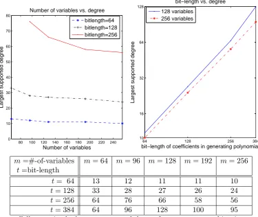
Figure 1: Supported degree vs. number of variables and bit-length of the generating polynomial, all tests were run in dimensionn= 128
7
How Homomorphic is This Scheme?
We ran some experiments to get a handle on the degree and number of monomials that the somewhat homomorphic scheme can handle, and to help us choose the parameters. In these experiments we generated key pairs for parameters n (dimension) and t (bit-length), and for each key pair we encrypted many bits, evaluated on the ciphertexts many elementary symmetric polynomials of various degrees and number of variables, decrypted the results, and checked whether or not we got back the same polynomials in the plaintext bits.
More specifically, for each key pair we tested polynomials on 64 to 256 variables. For every fixed number of variables m we ran 12 tests. In each test we encryptedm bits, evaluated all the elementary symmetric polynomials in these variables (of degree up to m), decrypted the results, and compared them to the results of applying the same polynomials to the plaintext bits. For each setting of m, we recorded the highest degree for which all 12 tests were decrypted to the correct value. We call this the “largest supported degree” for those parameters.
tested various dimensions from 128 to 2048 with a few settings oftandm, and the largest supported degree was nearly the same in all these dimensions. Thereafter we tested all the other settings only in dimensionn= 128.
The results are described in Figure 1. As expected, the largest supported degree grows linearly with the bit-length parameter t, and decreases slowly with the number of variables (since more variables means more terms in the polynomial).
These results can be more or less explained by the assumptions that the decryption radius of the secret key is roughly 2t, and that the noise in an evaluated ciphertext is roughly cdegree × √
#-of-monomials, where c is close to the Euclidean norm of fresh ciphertexts (i.e., c ≈ 9). For elementary symmetric polynomials, the number of monomials is exactly (degm). Hence to handle polynomials of degreedegwithmvariables, we need to settlarge enough so that 2t≥cdeg×√(degm), in order for the noise in the evaluated ciphertexts to still be inside the decryption radius of the secret key.
Trying to fit the data from Figure 1 to this expression, we observe thatcis not really a constant, rather it gets slightly smaller whentgets larger. Fort= 64 we havec∈[9.14,11.33], fort= 128 we havec∈[7.36,8.82], fort= 256 we getc∈[7.34,7.92], and for t= 384 we havec∈[6.88,7.45]. We speculate that this small deviation stems from the fact that the norm of the individual monomials is not exactly cdeg but rather has some distribution around that size, and as a result the norm of the sum of all these monomials differs somewhat from √#-of-monomials times the expectedcdeg.
Part II
A Fully Homomorphic Scheme
8
Squashing the Decryption Procedure
Recall that the decryption routine of our “somewhat homomorphic” scheme decrypts a ciphertext
c ∈ Zd using the secret key w ∈ Zd by setting b ← [wc]dmod 2. Unfortunately, viewing c, d as constants and considering the decryption function Dc,d(w) = [wc]dmod 2, the degree of Dc,d (as a polynomial in the secret key bits) is higher than what our somewhat-homomorphic scheme can handle. Hence that scheme is not yet bootstrappable. To achieve bootstrapping, we therefore change the secret-key format and add some information to the public key to get a decryption routine of lower degree, as done in [4].
On a high level, we add to the public key also a “big set” of elements{xi∈Zd : i= 1,2, . . . , S}, such that there exists a very sparse subset of the xi’s that sums up tow modulod. The secret key bits will be the characteristic vector of that sparse subset, namely a bit vector ⃗σ = ⟨σ1, . . . , σS⟩ such that the Hamming weight of⃗σ is s≪S, and ∑iσixi=w (modd).
Then, given a ciphertext c∈Zd, we post-process it by computing (in the clear) all the integers
yi def
= ⟨cxi⟩d (i.e., c times xi, reduced modulo d to the interval [0, d)). The decryption function
Dc,d(⃗σ) can now be written as
Dc,d(⃗σ) def=
[∑S
i=1
σiyi
]
d mod 2
again modulo d to the internal [−d/2,+d/2). We now show that (under some conditions), this functionDc,d(·) can be expressed as a low-degree polynomial in the bitsσi. We have:
[∑S
i=1
σiyi
]
d =
(∑S
i=1
σiyi
)
−d·
⌈∑
iσiyi
d
⌋
=
(∑S
i=1
σiyi
)
−d·
⌈ S ∑ i=1 σi yi d ⌋ ,
and therefore to computeDc,d(⃗σ) we can reduce modulo 2 each term in the right-hand-side sepa-rately, and then XOR all these terms:
Dc,d(⃗σ) =
(⊕S
i=1
σi⟨yi⟩2
)
⊕ ⟨d⟩2·
⟨ ⌈∑S
i=1 σi yi d ⌋ ⟩ 2 = S ⊕ i=1
σi⟨yi⟩2 ⊕
⟨ ⌈∑S
i=1 σi yi d ⌋ ⟩ 2
(where the last equality follows since d is odd and so ⟨d⟩2 = 1). Note that the yi’s and d are constants that we have in the clear, and Dc,d is a functions only of the σi’s. Hence the first big XOR is just a linear functions of the σi’s, and the only nonlinear term in the expression above is the rounding function⟨⌈∑Si=1σiydi
⌋⟩
2.
We observe that if the ciphertextc of the underlying scheme is much closer to the lattice than the decryption capability ofw, thenwcis similarly much closer to a multiple ofdthand/2. In the bootstrappable scheme we will therefore keep the noise small enough so that the distance fromcto the lattice is below 1/(s+ 1) of the decryption radius, and thus the distance fromwcto the nearest multiple of dis bounded belowd/2(s+ 1). (Recall thatsis the the number of nonzero bits in the secret key.) Namely, we have
abs([wc]d) = abs
([∑S
i=1
σiyi
]
d
)
< d
2(s+ 1)
and therefore also
abs
([∑S
i=1 σi yi d ]) < 1
2(s+ 1)
Recall now that theyi’s are all in [0, d−1], and therefore yi/dis a rational number in [0,1). Let p be our precision parameter, which we set to
p def= ⌈log2(s+ 1)⌉.
For everyi, denote byzithe approximation ofyi/dto withinpbits after the binary point.5Formally,
zi is the closest number to yi/d among all the numbers of the form a/2p, with a an integer and 0 ≤ a≤ 2p. Then abs(z
i− ydi) ≤2−(p+1) ≤1/2(s+ 1). Consider now the effect of replacing one term of the formσi·ydi in the sum above byσi·zi: Ifσi = 0 then the sum remains unchanged, and ifσi = 1 then the sum changes by at most 2p+1 ≤1/2(s+ 1). Since onlysof the σi’s are nonzero, it follows that the sum ∑iσizi is at most s/2(s+ 1) away from the sum
∑
iσiydi. And since the distance between the latter sum and the nearest integer is smaller than 1/2(s+1), then the distance between the former sum andthe same integer is strictly smaller than 1/2(s+ 1) +s/2(s+ 1) = 1/2. It follows that both sums will be rounded to the same integer, namely
⌈ S ∑ i=1 σi yi d ⌋ = ⌈ S ∑ i=1
σizi
⌋
5