An Adaptive Weighted Average (WAV) Reprojection Algorithm for Image Denoising

(1)

Western University Western University

Scholarship@Western

Electronic Thesis and Dissertation Repository

May 2019

An Adaptive Weighted Average (WAV) Reprojection Algorithm for

Image Denoising

Halimah Alsurayhi

The University of Western Ontario

Supervisor

Mahmoud El-Sakka

The University of Western Ontario Graduate Program in Computer Science

A thesis submitted in partial fulfillment of the requirements for the degree in Master of Science © Halimah Alsurayhi 2019

Follow this and additional works at: https://ir.lib.uwo.ca/etd

Part of the Theory and Algorithms Commons

Recommended Citation Recommended Citation

Alsurayhi, Halimah, "An Adaptive Weighted Average (WAV) Reprojection Algorithm for Image Denoising" (2019). Electronic Thesis and Dissertation Repository. 6196.

(2)

Abstract

Patch-based denoising algorithms have an effective improvement in the image

denois-ing domain. The Non-Local Means (NLM) algorithm is the most popular patch-based

spatial domain denoising algorithm. Many variants of the NLM algorithm have

pro-posed to improve its performance. Weighted Average (WAV) reprojection algorithm

is one of the most effective improvements of the NLM denoising algorithm. Contrary

to the NLM algorithm, all the pixels in the patch contribute into the averaging

pro-cess in the WAV reprojection algorithm, which enhances the denoising performance.

The key parameters in the WAV reprojection algorithm are kept fixed regardless of

the image structure. In this thesis, an improved WAV reprojection algorithm is

pro-posed, where the patch size is assigned adaptively based on the image structure. The

image structure is identified using an improved classification method that is based on

the structure tensor matrix. The classification result is also utilized to improve the

identification of similar patches in the image. The experimental results show that

the denoising performance of the proposed method is better than that of the original

WAV reprojection algorithm, as well as some other variants of the NLM algorithm.

(3)

Dedication

To my lovely parents

Aisha Alsurayhi, and Abdullah Alsurayhi

(4)

Acknowledgements

First and foremost, I would like to thank God Almighty for giving me the ability to

complete my thesis successfully. Without his blessings, this achievement would not

have been possible.

I would like to express my very great appreciation to Dr. Mahmoud El-Sakka, my

thesis supervisor, for his professional guidance and valuable support. His willingness

to give his time so generously has been very much appreciated.

My grateful thanks are also extended to my husband Khalid Nuli for his support

and encouragement throughout my study.

Finally, I wish to thank my friend, Seereen Noorwali, for her assistance in my

(5)

List of Figures

2.1 The strategy of the NLM algorithm in finding the similar patches [4],

the weight of q1, and q2 is larger than the weight of q3 as q1, and q2 have similar neighbourhood to the reference pixel p . . . 11

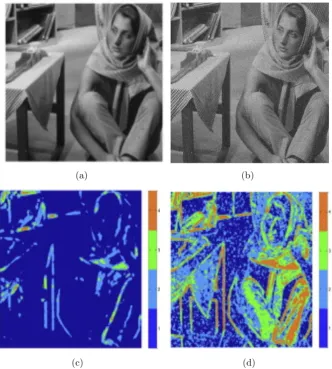
2.2 The improved classification results on Barbara image: (a) Original

image, (b) Noisy imageσ= 20. (c) The structure tensor classification, (d) The improved classification by Hu and Luo [17]. (Orange: texture

with little noise, green: medium region, light blue: texture with high

noise and dark blue is the flat region) . . . 17

2.3 The three basic steps of the WAV reprojection algorithm [34] . . . . 21

2.4 The difference between the (a) centred patches and (b) the decentred

patches in the gathering step [34] (The red patch is the reference patch) 22

2.5 The Gaussian kernel and the Flat kernel . . . 23

2.6 The difference between the influence zone in the centred patch (a),

and the decentred patch (b) [34] (The patch size W = 5, and the

searching window R=15) . . . 24

(9)

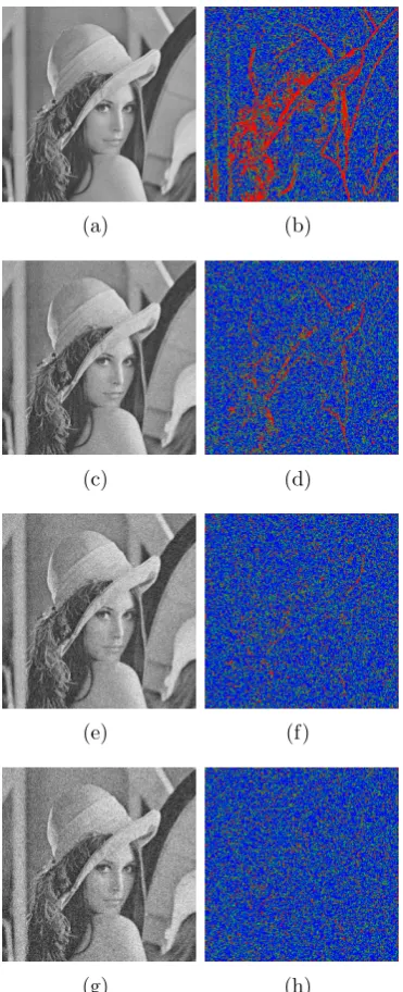
3.1 The classification results using the structure tensor on Lena image:(The

red color represents edge pixels, the blue color represents the smooth

pixels, and the green color represents texture/noise pixels) (a) Noisy

image σ = 10, (b) Classification of noisy image σ = 10, (c) Noisy imageσ= 20, (d) Classification of noisy image σ= 20, (e) Noisy im-ageσ = 30, (f) Classification of noisy image σ= 30, (g) Noisy image

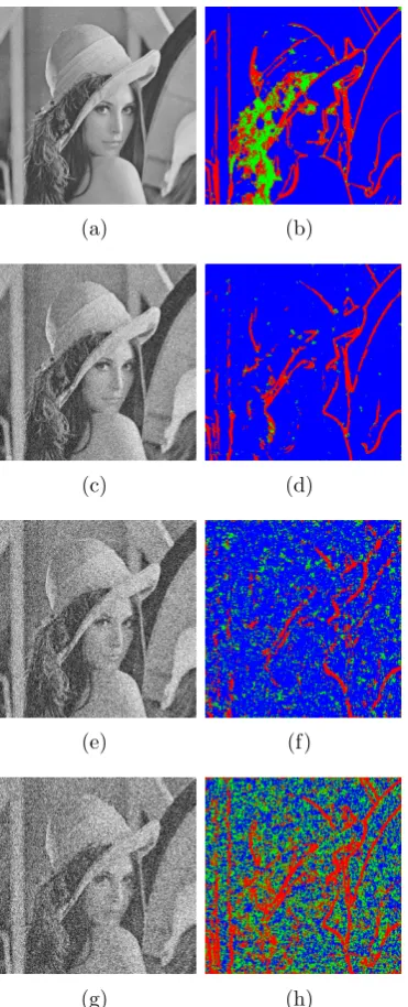
σ= 40, (h) Classification of noisy image σ= 40 . . . 30 3.2 The improved classification results on Lena image: (The red color

shows the edge pixels, the blue color shows the smooth pixels, and

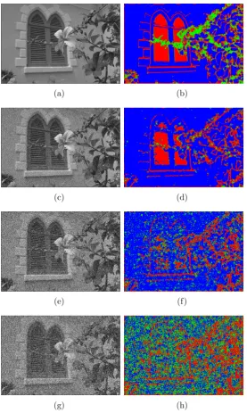
the green color shows texture/noise pixels) (a) Noisy image σ = 10, (b) Classification of noisy image σ = 10, (c) Noisy image σ = 40, (d) Classification of noisy image σ= 40, (e) Noisy image σ = 70, (f) Classification of noisy image σ = 70, (g) Noisy image σ = 100, (h) Classification of noisy imageσ = 100 . . . 33 3.3 The improved classification results on Window image image: (The red

color shows the edge pixels, the blue color shows the smooth pixels,

(10)

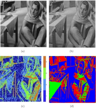
3.4 The classification results comparison on Barbara image: (a) Original

image, (b) Noisy image σ = 20, (c) The improved classification by Hu and Luo [17]. (Orange: texture with little noise, green: medium

region, light blue: texture with high noise and dark blue is the flat

region), (d) Our classification method: (The red color shows the edge

pixels, the blue color shows the smooth pixels, and the green color

shows texture/noise pixels) . . . 35

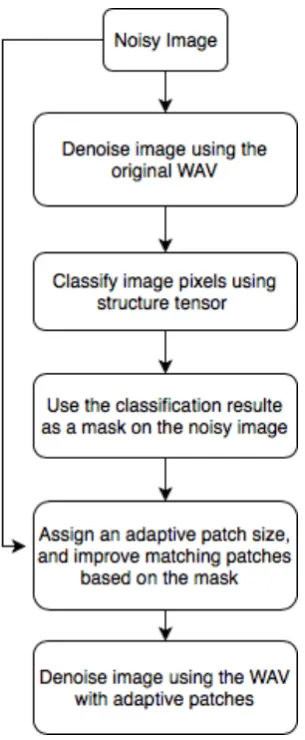
3.5 The basic steps of our improved method . . . 36

3.6 The Mean PSNR values of smooth areas in 25 different natural scene

images: (a) Noiseσ= 10 to 50, (b) Noise σ= 60 to 100 . . . 39 3.7 The Mean PSNR values of edge areas in 25 different natural scene

images: (a) Noiseσ= 10 to 50, (b) Noise σ= 60 to 100 . . . 41 3.8 The Mean PSNR values of texture areas in 25 different natural scene

images: (a) Noiseσ= 10 to 50, (b) Noise σ= 60 to 100 . . . 43 3.9 The performance of different patch sizes around the edges on Lena

image (noise σ = 10): (a) Original Image, (b) Denoised image using patch 5_×5, (c) Denoised image using patch 7_×7, (d) Denoised image

using patch 9_×9, (e) Denoised image using patch 11_×11, (f) Denoised

(11)

3.10 The performance of different patch sizes on texture part from Lena

image(noise σ = 10): (a) Original Image, (b) Denoised image using patch 5_×5, (c) Denoised image using patch 7_×7, (d) Denoised image

using patch 9_×9, (e) Denoised image using patch 11_×11, (f) Denoised

image using patch 13_×13. . . 46

3.11 The smooth part from Lena image . . . 47

4.1 The 10 images used in our experiments: (a) Lena image 512_×512, (b)

Man image 512_×512, (c) Couple image 512_×512, (d) Columbia image

480_×480, (e) Barbara image 720_×850, (f) Boats image 720_×576, (g)

House image 768_×512, (h) Light House image 512_×768, (i) Window

image 768_×512, (j) Woman image 512_×512 . . . 51

4.2 The mean PSNR values of the 10 images set in 10 different noise levels 54

4.3 The PSNR values of Window image in 10 different noise levels . . . . 55

4.4 The mean SSIM values of the 10 image set in 10 different noise levels 57

4.5 The SSIM values of the Window image in 10 different noise levels . . 58

4.6 The visual comparison of Window image with noiseσ= 10: (a) Origi-nal Image, (b) Noisy image, (c) Denoised image using NLM algorithm,

(d) Denoised image using WAV reprojection algorithm, (e) Denoised

image using Adaptive patch shape NLM algorithm, (f) Denoised image

(12)

using our proposed method . . . 61

4.10 Zoomed part from Window image with noise σ = 10: (a) Original Image, (b) Noisy image, (c) Denoised image using NLM algorithm,

(13)

4.14 The two horizontal lines used for intensity profile . . . 68

4.15 Difference in intensity profile when the NLM algorithm and our

pro-posed method are applied along line y = 230 . . . 69

4.16 Difference in intensity profile when the WAV reprojection algorithm

and our proposed method are applied along line y = 230 . . . 69

4.17 Difference in intensity profile when the adaptive patch shape NLM

(14)

4.18 Difference in intensity profile when the NLM algorithm and our

pro-posed method are applied along line y = 450 . . . 70

4.19 Difference in intensity profile when the WAV reprojection algorithm

and our proposed method are applied along line y = 450 . . . 71

4.20 Difference in intensity profile when the adaptive patch shape NLM

algorithm and our proposed method are applied along line y = 450 . 71

4.21 The PSNR performance of BM3D, the adaptive BM3D, and the

(15)

List of Tables

3.1 The mean PSNR values of smooth areas in 25 different natural scene

images using 10 different noise levels . . . 38

3.2 The mean PSNR values of edge areas in 25 different natural scene

images using 10 different noise levels . . . 40

3.3 The mean PSNR values of texture areas (or noise) in 25 different

natural scene images using 10 different noise levels . . . 42

3.4 The mean PSNR values of a part from Lena’s face and the background 46

4.1 The mean PSNR values of the 10 images set in 10 different noise levels 54

4.2 The PSNR values of Window image in 10 different noise levels . . . . 55

4.3 The mean SSIM values of the 10 image set in 10 different noise levels 57

4.4 The SSIM values of the Window image in 10 different noise levels . . 58

4.5 The PSNR performance of BM3D, the adaptive BM3D, and the

(16)

List of Abbreviations

NLM Non-Local Means

WAV Weighted Average reprojection algorithm

BM3D Block Matching and 3D collaborative filtering

DCT Discrete Cosine Transform

FFT Fast Fourier Transform

PSNR Peak Signal to Noise Ratio

(17)

Chapter 1 Introduction

Digital images are represented as a two-dimensional array of pixels. So, each pixel

defined asf(x, y), wheref is the grey level value or the pixel intensity, and (x, y) are the spatial coordinates of the image pixel. Digital images might be contaminated by

noise during acquisition or transmission processes, which affected the original image

signals. Image noise could cause problems in some other image processing stages

such as image segmentation or image recognition. Therefore, image denoising is an

important process to restore the original clean image signals from its observed noisy

signals.

Over the years, variant image denoising approaches have been proposed. Most of

them achieved denoising by averaging in a way or another. This averaging may be

performed in spatial domain such as Gaussian Smoothing model [15] [20], Anisotropic

Filtering (AF) [27] [37], and Total Variation minimization [32] [31]; or in the

(18)

In recent years, patch-based denoising algorithm has drawn a lot of attention in the

image denoising field, where the neighbouring patches (image block) in a specific

search window participate in the denoising process for a certain reference patch in

the noisy image. This helps to find the best estimate for the original image signal

from its noisy signal.

1.1 Motivation

Patch-based denoising algorithms have become extremely popular in the image

de-noising field. They take the advantage of the similarity within the images, where

image signals are restored by performing averaging between the similar patches in the

image. Buades et al. [4] have introduced a patch-based algorithm called Non-Local

Means (NLM) for image denoising.

Variants of NLM algorithm have been proposed to improve its performance by

adaptively selecting some of the internal parameters. Some of these variants have

assigned the smoothing parameter adaptively based on the image structure [7] [36]

[39], or based on the noise level [41]. Some other variants are based on selecting the

patch size adaptively using the image structure [17] [23] [40]. Besides the adaptive

patch size, Deledalle et al [10] proposed a shape adaptive patches to address the

problem of the halo of noise around the edges. Some other variants have improved

the NLM algorithm by improving the method of computing the similarity between

(19)

One of the significant improvements in the patch-based denoising methods is the

WAV reprojection algorithm [34] which moved the reprojection method from the

patch space to pixel space. The WAV reprojection algorithm takes the advantage

of the whole patch, i.e., all pixels in the patch are exploited, which enhances the

denoising performance.

The key parameters of the WAV reprojection algorithm have kept fixed, regardless

of the image structure. So, one of our focus is to improve the performance of the

WAV reprojection algorithm by assigning anadaptivepatch size based on the image structure. Also, we propose to improve the WAV reprojection algorithm by

improv-ing matchimprov-ing the similar patches.

1.2 Thesis contribution

Edges are preserved better with a small patch size while smooth regions have

bet-ter denoising performance with large patch size [39] [40]. In the WAV reprojection

algorithm, the patch size has set to be fixed regardless of the image structure. So,

we propose anadaptive patch size WAV reprojection algorithm that is based on the image structure. The image pixels are classified based on our improved classification

method. We improve the classification method provided by [40] that is based on

the eigenvalues of the structure tensor matrix. The improved method is derived by

combining it with the discontinuity indicator [39] that classifies the image pixel into

(20)

amount of noise that affected the classification procedure. We classified the image

pixels into three classes: smooth, edge, texture / noise. The classification result is

then used as a mask on the noisy image to assign the patch size adaptively

Moreover, we used the classification scheme to improve the method of finding

similar patches. Two patches consider being similar only if they are from the same

class. Our proposed method has improved the original WAV reprojection algorithm

in term of PSNR and SSIM performance. Also, it has better preserved edges and

texture in the image.

1.3 Thesis Outline

Our thesis consists of five chapters. This chapter, Chapter 1, is an introductory chapter. In Chapter 2, we discuss in detail some patch-based image denoising algorithms. Our methodology is presented inChapter 3 with some experiments to assign the best patch size for each class. InChapter 4, we present the experimental results of our method, and we compare it with some other competitive methods.

(21)

Chapter 2 Background

Digital images are often affected by unwanted signals (noise) during the acquisition

or transmission processes. Image noise can cause problems in further image

process-ing processes such as identification, segmentation. Noise comes in different models.

Different methods are used to handle each noise model. This chapter focuses on

Ad-ditive White Gaussian Noise, which is the most common noise considered in image

processing. Different denoising algorithms to address this type of noise are discussed.

2.1 Additive White Gaussian Noise

The additive noise occurs when the noise signal is added to the original image signal,

it is generally modelled as:

(22)

wherev is the noisy image, uis the clean image, andn is the noise. In the Additive White Gaussian Noise, the noise has a uniform (constant) power over all frequencies

with amplitude following the Gaussian distribution. So, for a Gaussian variable z

the probability density function is:

p(z) = _√1

πσe

−(z₂−_σµ2)2 _(2.2)

whereµ is the mean value, σ is the standard deviation, and σ2 _{is the variance of} _z_, andz is the amount of noise.

2.2 Noise Level Estimation

There are different methods to estimate the noise variance. They generally classified

as filtered based, patch-based, and statistical based. The filtered based approaches

estimate the noise by a pre-filter process using a low pass filter to suppress the

image structure [35] [19]. Then, the noise is estimated as the difference between

the filtered image and the noisy one. The patch-based noise estimation decomposes

the image into patches. Then, the homogeneous patches are used to estimate the

noise level [24] [25]. The main issue in patch-based methods is how to specify the

homogeneous patches. Also, some patch-based methods require high computation

load as it estimates the noise in an iterative way. The statistical methods analyse the

local variance distribution. Their results are more robust as the statistical methods

used are insensitive to outliers [2] [14].

(23)

used one of the filtered-based noise level estimations. It is just a simple method that

doesn’t require any high computation load (See Section 3.2).

2.2.1 Fast Noise Level Estimation

The fast noise level estimation [19] includes two steps, convolution and averaging.

The following Laplacian mask is applied first on the noisy image.

The noise estimation is the mask operation using the mask N, which has zero mean and variance (42 _{+ 4}_×₍₂₎2 _{+ 4}_×₍₁₎2₎_σ2

n = 36σ2n. The variance of the

convolution of the N on the noisy image I gives an estimate of 36 σ2

n at each pixel.

So, the averging is applied to get an estimated noise varianceσ2

n as follow:

σ_n2 = 1

36(W ₋2)(H₋2)

X

imageI

(I(x, y)_∗N)2 (2.3)

(24)

2.2.2 Patch-based Noise Estimation

The homogenous patches are targeted in the patch-based noise estimation [24] [25].

So, the image is first decomposed into a number of patches. The homogeneous

patches are then distinguished as the patches with the smallest standard deviation

because they have the least change of intensity among decomposed patches. As

intensity variation of the homogeneous patches is mostly caused by the noise, the

noise level is estimated from the selected patches. Patch-based noise estimation

methods overestimate the noise level in the small noise levels, and they underestimate

the noise in the large noise levels.

2.2.3 Statistical-based Noise Estimation

The analysis of the local variance distribution is used to estimate the noise in the

statistical-based method [2]. The image is decomposed into a number of small blocks.

Then, the local intensity variance of each block is calculated. The variance of all

blocks are averaged to estimate the noise variance. The size of the blocks used

should be as small as possible (e.g. 2_×2)

2.3 Image Denoising

Image denoising is an important process to restore the original image signals from the

noisy ones. The main objective in image denoising is to reduce noise while preserving

edges and textures.

(25)

them achieved denoising by averaging in a way or another. This averaging may be

performed in the spatial domain, or in the frequency domain. In the spatial domain,

the spatial neighbouring pixels are considered in denoising, such as the convolution

of the Gaussian kernel [15]. In the frequency domain, the image is transformed to the

frequency domain like Fourier transform [8], or Wavelet transform [26]. The filtering

is performed in the frequency domain, then the inverse of the transform is applied

to get the denoised image.

Recently, patch-based denoising algorithms have became extremely popular in the

denoising field. They take the advantage of the similarity within the images. So, the

averaging is performed based on the similarity between image patches. Buades et

al. [4] have introduced the patch-based method for image denoising. They developed

the NLM (Non-Local Means) algorithm. Other patch-based denoising algorithm that

has the best performance results in denoising is BM3D [9]. In this chapter, various

patch-based denoising algorithms are discussed.

2.4 Patch-Based Denoising Algorithm

Natural scene images have a high degree of similarity, which means that each small

block has many similar blocks in the same image. Patch-based denoising algorithms

(26)

2.4.1 Non-local Means Algorithm

The (NLM) algorithm [4] estimates the original image signal by considering the

neighbouring area of the current processed pixel. For each pixel, they find all nearby

similar patches in the image that match the patch around the current processed

pixel (See Figure 2.1). Similar patches are chosen under some conditions based

on the similarity in the gray-level value, the geometrical configuration in a whole

neighbourhood, and how far they are from the current pixel. Then, the weighted

average of all centred pixels in all similar patches is calculated. Those weights depend

on the similarity between the patches. That is, pixels that their surroundings are

similar in the gray-level values to the current processed one have more weights than

other pixels, and closer pixels have more weight than the faraway one.

For a noisy imagev, wherev =_{v(i)_|i_∈I_}, iis the coordinate of a pixel within the image, the NLM for a pixel at location i,

N L[v](i) =X

j∈i

w(i, j)v(i) (2.4)

wherew is the weight, and it depends on the similarity between pixels at locationsi

andj. Euclidean distance has been used to calculate the distance between patches. Each weightw has to be less than or equal 1 and larger than or equal to 0, while the total of all weights has to equal 1. The weight is calculated as follow:

w(i, j) = 1

Z(i)e

−||v(Ni)−v(Nj)|| 2 2,a

(27)

whereZ(i) is the normalizing constant, and it is defined as:

Z(i) =X

j e−||

v(_Ni)−v(_Nj)||2₂_,a

h2 (2.6)

where v(Ni) and v(Nj) are the intensity gray level vectors of the neighbourhood of

pixels i and j respectively. _||v(Ni)−v(Nj)||22,a is the Euclidean distance between

patches surrounding pixels i and j, a is the standard deviation of the Gaussian kernel and it is greater than 0, and h is the constant that control the decay of the exponential weight function (smoothing parameter).

Fig. 2.1 – The strategy of the NLM algorithm in finding the similar patches [4], the weight of q1, and q2 is larger than the weight of q3 as q1, and q2 have similar neighbourhood to the reference pixel p

2.4.2 Adaptive Smoothing Parameter NLM

(28)

for smooth and edges areas, degrades the denoising performance of the NLM

algo-rithm. Denoising smooth areas with the NLM algorithm works better with a larger

smoothing parameter while at edges and textures areas using smaller smoothing

parameter produces better results. Thus, different methods have been proposed to

adaptively select the smoothing parameter for each pixel based on the image features.

Chen and Yang [7] have proposed a method to select the smoothing parameter

adaptively. In their method the smoothing parameter is assigned based on the local

grey-level variance of the image pixel. The local grey-level variance identifies the

image structure, it distinguishes between the noise and the image edge or texture.

The local grey-level variance is provided by:

σ_l2(x, y) = 1

D2₋₁ D−1

2

X

i,j=−(D₂−1)

[I(x+i, x+j)₋ml(x, y)]2 (2.7)

Where D is the size of the sliding window, and ml is the local mean of the pixels

in the window. Based on the resulted classification, a small smoothing parameter is

assigned for pixels on edges, or texture areas, and a large smoothing parameter is

assigned for pixels on smooth areas.

Verma and Pandy [36] provided another method to choose the smoothing

param-eter adaptively. They classify the image regions using the Grey relational analysis,

which is related to the theory of the grey system [11]. The Grey relational analysis

(29)

fac-tor to all other facfac-tors in a system. The grade of the grey relations between image

patches is calculated using Grey relational analysis. Then, an adaptive smoothing

parameter is assigned for each pixel based on the resulted classification.

One more method to assign an adaptive smoothing parameter is based on the

discontinuity indicator [39]. A novel discontinuity indicator is proposed to detect

image structure; it also distinguishes between edges and noise. The discontinuity

indicator is derived from the eigenvalues of the structure tensor matrix [22]. It is

obtained as the difference between the two eigenvalues for each pixel.

The resulted discontinuity indicator is used to classify image pixels. If the

dis-continuity indicator is large, the pixel considered to be on edge. If it is small and

the two eigenvalues are also small, the pixel considered to be on smooth region.

The pixel is noise if the discontinuity indicator is small and the two eigenvalues are

large. Hence, an adaptive smoothing parameter is chosen for each pixel based on the

resulted classification.

Zhu et.al. [41] proposed an improved NLM by applying the NLM method twice.

First, the noise variance is estimated using the weak textured patch noise estimation

[24]. The weak textured patches are selected based on the image gradient. Then, the

Principle Component Analysis (PCA) is applied on the selected patches to attain

the estimated noise level. After that, the Non-Local means method is applied on the

noisy image using an adaptive smoothing parameter based on the estimated noise

variance to get the basic estimate. The final estimate is then obtained by applying

(30)

removed in the first step.

Adaptive NLM using Weight Thresholding

Khan and El-Sekka proposed the NLM using Weight Thresholding [21]. Their

method is performed as a two-step approach. The basic estimate is generated in

the first step by thresholding the weights of the pixels within the searching area.

All weights above the threshold value are unchanged, but the weights less than the

threshold are assigned to zero, thus those pixels are removed from the weighted

averaging process. In the second step, the weighted thresholding NLM is applied

once again but with different smoothing strength. The threshold value is adaptively

assigned based on the noise level.

2.4.3 Adaptive Patch Size NLM

Adaptive patch size based on image structure

The patch size has set to be fixed in the original NLM algorithm. Using a variable

patch size has a significant improvement on the performance of the NLM method.

Edges are preserved better with a small patch size while smooth regions have better

denoising performance with large patch size. Various adaptive patch size NLM

de-noising algorithm are proposed to overcome the inefficacy of the traditional NLM.

Zeng et al. [40] have proposed an adaptive patch size NLM algorithm. They use the

structure tensor to classify the image into smooth and texture regions. The difference

between the two eigenvalues of the structure tensor is calculated. If the difference

(31)

and a large patch size is set to estimate its original value. On the other hand, if the

difference is small, the pixel is considered to be on a texture area and hence a small

patch size is set to estimate its original value.

Hu and Luo [17] has also improved the NLM algorithm by adaptively select the patch

size based on image structure. They use the local geometry of the image and the

noise variance to drive a new metric,

R(i) =f(i)

λ2 1−λ22

λ2 1+λ22

(2.8)

where f(i) is a feature detector based on the image histogram, λ1 and λ2 are eigenvalues of the structure tensors that used to classify the image structure. This

composed metric classifies the image into four regions (c1, c2, c3, and c4) based on their relations to three bin values T1 = 90%, T2 = 70%, and T3 = 30% (See Figure 2.2), i_∈                       

c1 R(i)≥T1

c2 T2 < R(i)< T1

c3 T3 < R(i)≤T2

c4 R(i)≤T3

(2.9)

where c1 represents texture region with a small value of noise variance, c2 is the medium region that has even smaller noise variance and less structure,c4 is the flat region, and c3 represents region with textures and high value of noise. Then, dif-ferent patch sizes are applied to each region. The largest patch size is assigned to

(32)

tex-ture. The patch size increases gradually inc1andc2 as the regions have less texture .

Lan et al [23] have also proposed an adaptive patch size NLM scheme based on

region homogeneity. In their method, the patch size and the searching window sizes

are assigned adaptively depending on the local scale measure. The local scale finds

the homogeneous regions in the image according to the image structure [33]. The

homogeneity range is large inside regions and it becomes smaller on edges. So, the

local scale is computed for each pixel, then the patch size and the searching window

size are assigned accordingly.

Adaptive Patch Shape NLM

Besides the adaptive patch size, Deledalle et al [10] proposed a shape adaptive patches

to address the problem of the halo of noise around the edges. Various shapes have

been used including square, disk, pie, slices, and bands. The variety in shapes is

applied to handle the geometrical structure of the image. Fast Fourier Transform

(FFT) is used to deal with the different shapes of patches. For aggregation, the same

weight is assigned for all patch shapes. The proposed algorithm has a noticeable

improvement for the noise halo.

The Patch Size and the Noise Variance

The knowledge of the noise variance improves the performance of the NLM algorithm.

(33)

(a) (b)

(c) (d)

(34)

using larger patches have better denoising results, i.e, larger patch sizes allow better

discrimination between patches [13]. Thus, it is better to use large patch size for its

robustness to noise. On the other hand, choosing large patch size prevents finding

similarities for the small details, also it degrades the denoising performance around

edges. Thus, the author suggests assigning an adaptive smoothing parameterhwith a global patch size to overcome the issue of smoothing the edges.

2.4.4 NLM with Improved Similarity Computation Method

The Euclidean distance with the geometric image structure are used to find similar

patches. This method is based only on the noisy image, which might not provide

the structure similarity efficiently, especially with high noise variance. Thus, other

approaches have been provided to improve the similarity method.

Curvelet based NLM algorithm

In the curvelet based NLM [38], the Curvelet transform is first applied on the noisy

image. The Curvelet transform is a directional multi-scale transform that produces

an optimal representation of image features like edges [12]. Similar patches are

determined based on the different levels of the resulted reconstructed images by the

Curvelet transform beside the noisy image. The final denoised image is obtained by

(35)

K-Means Clustering based NLM

The K-means clustering is combined with NLM algorithm to improve matching the

similar patches [28]. The K-Means algorithm classifies the image pixels into a number

of clusters based on the distance of their intensities from the centroid [16]. First, the

noisy image is smoothed using a Gaussian smoothing filter. Gaussian filtering [15]

recovers the image signals by applying the convolution of the Gaussian kernel on the

noisy imageI0.

I(x, y) =I0(x, y)∗G(x, y) (2.10)

where

G(x, y) = 1 (4πh2₎e

−|₄x_h|22 (2.11)

The K-means technique is then applied on the smoothed imageI to create the mask imageIm.

Im = K

X

i=1

X

xj∈si

kxj−µik2 (2.12)

Whereµis the centroid or the mean of the cluster, and k is the number of the clus-ters and it depends on the image structure. The resulted imageIm is used as a mask

for the noisy image to improve matching the similar patches. Finally, the denoised

image is obtiend as the weighted average of pixels in the similar neighbourhood Ω

within the cluster nas follow:

N L[vn](i) =

X

j∈Ω

(36)

DCT-Based Non-Local Means

In order to improve the patch similarity, the spatial distance between patches is

replaced by the distance between the discrete cosine transform (DCT) [1] coefficients

in the frequency domain [18]. The neighbourhood patches are transformed from

the spatial domain to the DCT frequency domain. Then, the DCT coefficients are

obtained through the Zigzag scan. Consequently, the weight in the NLM method is

replaced by:

w(i, j) = 1

Z(i)e −Pd

k=1

(_Cd(_Ni)_k−_Cd(_Nj)_k)2

h2 (2.14)

whereCd(Ni)k is the kth DCT coefficient of the neighbourhood of the subspace Ni, d_∈[1, M] where M is number of pixels in Ni, Z is the normalization factor, and h

is the Gaussian smoothing parameter.

2.4.5 Weighted Average Reprojection (WAV)

The Weighted Average (WAV) Reprojection algorithm is one of the significant

im-provements in the patch-based denoising methods. WAV reprojection algorithm [34]

has improved the reprojection method from the patch space to pixel space. The

de-noising is performed in three basic steps: collecting the similar patches, performing

the denoising for each patch, and reprojecting the denoised patch to the pixel domain

(37)

Fig. 2.3 – The three basic steps of the WAV reprojection algorithm [34]

In the first step, the chi-squared distributionχ2_{in conjunction with the Euclidean} distance is used to test the similarity between patches. Two patches are considered

to be similar if the Euclidean distance between them is less than the quantile of

χ2₍_W2_{). To estimate a pixel} _x _{after the grouping step, the weighted average of the} different estimators ofx in all patches pixelx is belong to is calculated.

ˆ

IW av(x) = W2

X

i=1

βiPˆi(W2−i+ 1) (2.15)

The weight βi is based on minimizing variance between patches. Because WAV

reprojection algorithm uses the flat kernel,βiis proportional to the number of patches

used to estimate ˆPi, and PW

2

i=1βi = 1.

Only the central pixel in each patch is used to estimate the current processed pixel

in the original Non-local means algorithm, which degrades the performance of the

(38)

(a)

(b)

Fig. 2.4 – The difference between the (a) centred patches and (b) the decentred patches in the gathering step [34] (The red patch is the reference patch)

takes the advantage of the whole patch, i.e., all pixels in the patch are exploited,

which enhances the denoising performance. The NLM algorithm performs poorly

around edges because the patches centred on the edges have a few similar patches.

The decentred patches is used in the WAV reprojection algorithm to enhance the

denoising performance around the edges. The decentred patches have more similar

patches than the centred patch, especially around the edges. Figure 2.4 shows the

number of patches that could be considered to denoise the pixels near the edges.

The WAV reprojection algorithm allows a faster implementation for two reasons.

(39)

the flat kernel all candidates have the same weight while Gaussian requires more

calculations as the weight varies from candidate to another. The flat kernel has an

advantage also in the denoising performance. it minimizes the problem encountered

by the Gaussian kernel in NLM algorithm when the searching window is too large.

More candidates are considered in the weight, and affects the impact of the good

candidates. The flat kernel robustifies the estimator by hard thresholding the small

coefficients .

Fig. 2.5 – The Gaussian kernel and the Flat kernel

The second reason is related to the searching window size, WAV reprojection

al-gorithm has good results with a small searching window size, e.g., (searching window

= 9). The influence zone is wider as the patches are decentred (See Figure 2.6) .

(40)

(a) (b)

Fig. 2.6 – The difference between the influence zone in the centred patch (a), and the decentred patch (b) [34] (The patch size W = 5, and the searching window R=15)

2.4.6 Image Denoising with Block-Matching and 3D

Collab-orative Filtering(BM3D)

BM3D [9] is one of the significant improvements in the patch-based denoising

ap-proach. It consists of two filtering steps; the hard thresholding filtering [5] that gives

the basic estimate, and the Wiener filtering [30] which produces the final estimate

(See Figure 2.7). Each step includes three operations: grouping, collaborative

filter-ing, and aggregation.

In the grouping operation, each reference block is compared with other blocks in the

image. The Euclidean distance is calculated, and the similar blocks are chosen if the

distance is less than a specified threshold.

SxR =

x_∈X_|d(ZxR, Zx)< τmatch

(41)

Then, all matched blocksSxRare stacked to form a 3D arrayZSxR. A 3D transfor-mation τ3D is then applied on the 3D array ZSxR to create a sparse representation. The hard thresholding is applied on the transform coefficients, which resulted in

multiple estimates for each pixel because the estimates may overlap. So, each

esti-mate is given a weight which is inversely proportional to the number of the non-zero

coefficients. In the aggregation operation, a weighted average of all estimates are

calculated to attain the basic estimate of the image.

In the second filtering step, the Weiner filtering is applied on the stacked local

esti-mates ˆYSxR that resulted from the hard thresholding step, and the stacked matched blocks from the noisy image. Then, the weighted average is calculated to get the

final estimate of the image.

Fig. 2.7 – The two steps of the BM3D algorithm [9].

Although BM3D has an effective improvement on the patch-based denoising

(42)

BM3D using an Adaptive Thresholding

In order to improve the thresholding process, an adaptive hard-thresholding is

as-signed in the hard thresholding step [3] of the BM3D Method. The adaptive

hard-thresholding is selected based on the geometric and luminance distance similarities

between patches. When a patch is geometrically far from the reference patch, more

thresholding is assigned to the patch transforming coefficients. The collaborative

Weiner filtering step is also improved by assigning more weights for similar patches.

They use weights for the 3D array patches. More weights are assigned for similar

patches. PSNR is used as a patch similarity measure for selecting those weights.

2.5 Conclusion

This chapter discussed different patch-based denoising algorithms. Also, different

variants of the NLM algorithm are described. They improved the NLM algorithm

by the adaptation selection of some internal parameters in the NLM scheme, or by

improving the similarity computation method. In addition, some other algorithms

that have significant improvements in the patch-based domain are discussed. In our

research we focus on the WAV reprojection algorithm. we studied its performance

(43)

Chapter 3 Methodology

WAV reprojection algorithm is one of the most powerful patch-based denoising

algo-rithms. It is a simple and effective method that performs the denoising in the spatial

domain. Unlike the NLM algorithm, all the pixels in the patches are exploited in

the WAV reprojection algorithm. A fixed patch size is used in the denoising process.

The similarity between patches is calculated using the Euclidean distance between

patches.

In our thesis, the patch size is assigned adaptively based on the image structure.

The image structures are identified using the structure tensor matrix. It classifies

the image pixels into three classes. In addition, the classification results are used to

improve matching similar patches. Patches similar to the reference patch contribute

(44)

3.1 Improved WAV Reprojection Algorithm

The prior knowledge about the image structure helps to set the parameters properly.

Edge information is preserved better with a small patch size, while smooth regions

have better denoising performance with large patch size. In the WAV reprojection

algorithm, the patch size has set to be fixed regardless of the image structure.

In our research, we target setting the patch size adaptively based on the image

structure to enhance the denoising performance. Thus, the image pixels need to be

classified first. We have used our improved method to classify the image pixels. The

next section explains in details our improved classification method.

3.1.1 The Improved Classification Method

The image pixels are first classified using the eigenvalues of the structure tensor

matrix [22]. The structure tensor matrix is defined as follow:

Tσ =

 

j11 j12

j21 j22

 

=

 

 Gσ∗(gx(i, j))

2 _G

σ∗gx(i, j)gy(i, j) Gσ_∗gy(i, j)gx(i, j) Gσ_∗(gy(i, j))2

 

 (3.1)

where gx and gy are the gradients information in x and y directions, and Gσ is

the Gaussian kernel. Then, the two eigenvalues are calculated:

λ1 = 1 2

j11+j22+

p

(j11−j22)2+ 4j122

(3.2)

λ2= 1 2

j11+j22−

p

(j11−j22)2+ 4j122

(45)

where j11 = Gσ ∗(gx(i, j))2, j22 = Gσ ∗(gy(i, j))2, and j12 = Gσ ∗gx(i, j)gy(i, j).

We follow the classification methods provided by [39] [40] to classify the image into

three regions. The absolute difference between the two eigenvaluesλ1 andλ2 is then calculated.

λ= _|λ1−λ2| (3.4)

Then, the following classification scheme is used to classify image pixels:

(i, j)_∈

                      

c1 λ(i, j)≤λ2(λ1−_nλ2)

c2 λ(i, j)≤λ22(λ1_n−λ2)

..

cn λ(i, j)≤λ2n(λ1_n−λ2)

(3.5)

This classification is inaccurate, as some pixels may belong to more than one

class. Also, it fails to classify the image pixels in the high noise levels, Figure 3.1

shows the classification result, where the red color represents edge pixels, the blue

color represents the smooth pixels, and the green color represents texture/noise

pix-els. In noise σ = 40, we can notice the described method fails to define the image structure.

Thus, we propose to improve the classification in Equation 3.5 by combining

it with the discontinuity indicator provided by Zeng et.al. [39]. The discontinuity

(46)

(a) (b)

(c) (d)

(e) (f)

(g) (h)

Fig. 3.1 – The classification results using the structure tensor on Lena image:(The red color represents edge pixels, the blue color represents the smooth pixels, and the green color represents texture/noise pixels) (a) Noisy imageσ= 10, (b) Classification of noisy image σ = 10, (c) Noisy image σ = 20, (d) Classification of noisy image

(47)

pixel is considered to be on an edge. If λ(i, j) is small and the two eigenvalues are also small, the pixel is considered to be on a smooth region. The pixel is noise if

λ(i, j) is small but the two eigenvalues are large.

In our method, we classify the image pixels into three classes based on a comparison

that made upon the two eigenvalues of the structure tensor matrix. We compare the

two eigenvalues of each pixel in each resulted class from Equation 3.5 with a specified

threshold value. If the two eigenvalues are smaller than thethreshold, the pixel is considered to be in a smooth area. If the maximum eigenvalueλ1 is larger than the

threshold and the minimum eigenvalue λ2 is smaller than the threshold, the pixel is considered on edge. The pixel is on texture or a noise if the two eigenvalues are

larger than the threshold.

(i, j)_∈

              

Smooth λ1 < τ, λ2< τ

Edge λ1 > τ, λ2< τ

T exture/N oise λ1 > τ, λ2> τ

(3.6)

where τ is the threshold value, and it has set to be 40.

In addition, we apply a preprocessing step to improve the classification results.

The image is denoised first using the original WAV reprojection algorithm. This

step has improved the classification result, especially at the low noise levels. The

texture areas can be classified as a third class when the noise level is less than 30.

However, when the noise level is high, the third class represents noise. Moreover, our

classification method has identified the image structure even when the noise level is

(48)

Figures 3.2 ,3.3 present our classification results on two different natural scene

images. One of them have mostly smooth regions(Lena), and the other one has more

texture region (Window). The classification results are presented with different noise

levels (σ= 10, σ= 40, σ= 70, σ= 100). The blue color presents the smooth areas, the red color presents the edges, and the green color presents the texture or noise

areas. When the noise level is low (σ= 10), the green color shows the texture only. While texture and noise are presented in green color when noise level is high (σ= 40,

σ= 70, andσ= 100). As the noise increase, the texture pixels tend to be presented as smooth pixels because the texture areas are blurred due to the denoising step.

However, our method has identified the edges even if the noise level is high.

Our improved classification method has better results than the method described in

Section 2.4.3. The noise signals could be distinguished from the original image signal,

while in their method the regions classified as texture with low noise or texture with

high noise. In the smooth region, if there is a noise, they just handle it as texture

with high noise. Figure 3.4 shows the comparison between our classification method

(49)

(a) (b)

(c) (d)

(e) (f)

(g) (h)

(50)

(a) (b)

(c) (d)

(e) (f)

(g) (h)

(51)

(a) (b)

(c) (d)

(52)

Fig. 3.5 – The basic steps of our improved method

3.1.2 The Improved WAV Reprojection Method

Figure 3.5 shows the block diagram of the proposed scheme. After the classification

step, we used the resulted classification as a mask on the noisy image. The improved

method is then obtained as follow:

(53)

averaging process only if their central pixels belong to the same class. That decreases

the number of un-similar patches from contributing in the averaging process.

In addition, an adaptive patch size is assigned to each pixel based on the class the

pixel is belong to. A large patch size is assigned to pixels on smooth areas, and a

small patch size is assigned to pixels on edges. For the texture, a smaller patch size

is assigned.

3.2 Selecting the patch size

In our experiments, we targeted natural scene images. We used 25 natural scene

images to select the best patch size for each class. The images are contaminated by

additive white Gaussian noise with 10 different levels of noise to assess the

perfor-mance of each class at each noise level and when using different patch sizes. Then,

the resulted mean PSNR values are used to assign the best patch size for each class.

We used patch sizes 5_×5, 7_×7, 9_×9, 11_×11, and 13_×13. The searching window

size has set to be fixed as 9_×9. The mean PSNR values of the 25 images in each

(54)

Noise level 5_×5 7_×7 9_×9 11_×11 13_×13

10 37.16 37.27 37.31 37.21 37.00

20 33.12 33.28 33.35 33.36 33.32

30 30.74 30.96 31.03 31.04 31.02

40 29.13 29.40 29.48 29.50 29.49

50 27.86 28.19 28.28 28.30 28.30

60 26.90 27.28 27.39 27.41 27.40

70 26.14 26.58 26.70 26.72 26.72

80 25.48 25.95 26.07 26.10 26.10

90 24.90 25.40 25.53 25.56 25.56

100 24.34 24.88 25.03 25.06 25.06

Mean 28.58 28.92 29.02 29.03 29.00

Table 3.1 – The mean PSNR values of smooth areas in 25 different natural scene images using 10 different noise levels

Figure 3.6 shows the bar chart of the mean PSNR comparison between the

dif-ferent patch sizes on the smooth areas. The results show that the smooth areas have

the best mean PSNR performance in noise level 10 when the patch size of 9_×9 is

used (See Table 3.1). The patch size 11_×11 have the best mean PSNR value in the

noise levels from 20 to 60. In noise levels more than 70, both patch sizes 11_×11 and

13_×13 have the best performance, but the algorithm with small patch size executes

(55)

(a)

(56)

Figure 3.7 plots the mean PSNR comparison when using different patch sizes on

the edge areas. The PSNR values are also reported in Table 3.2.The results show

that the patch size 5_×5 has the best mean PSNR performance in noise level 10.

Noise levels from 20 to 90 have the best results when the patch size of 7_×7 is used.

Patch 9_×9 has the best results when the noise level is 100. The average in all noise

levels shows that the best mean PSNR value for pixels on edges is when the patch

7_×7 is used.

Noise level 5_×5 7_×7 9_×9 11_×11 13_×13 10 32.81 32.62 32.22 31.85 31.58

20 28.46 28.60 28.54 28.34 28.11

30 25.70 25.82 25.77 25.64 25.46

40 23.81 23.87 23.78 23.63 23.44

50 22.47 22.48 22.37 22.21 22.02

60 21.59 21.60 21.48 21.32 21.14

70 20.98 21.02 20.93 20.79 20.64

80 20.68 20.78 20.72 20.61 20.49

90 20.49 20.66 20.64 20.56 20.47

100 20.41 20.65 20.68 20.64 20.57

Mean 23.74 23.81 23.71 23.56 23.39

(57)

(a)

(58)

Table 3.3 shows the PSNR comparison for the texture/noise pixels for different

patch sizes. Figure 3.8 presents the bar chart of the resulted mean PSNR values.

The results show that the patch size of 5_×5 has the best mean PSNR performance

in noise levels less than or equal to 30. In nose level 40, patch size 9_×9 has the best

mean PSNR performance. In the noise levels between 50 and 90, the patch size of

11_×11 has the best results. Both patch sizes 11_×11 and 13_×13 perform the same

in the noise level 100.

Noise level 5_×5 7_×7 9_×9 11_×11 13_×13 10 29.47 29.05 28.78 28.63 28.56

20 25.25 24.89 24.61 24.43 24.34

30 23.29 23.18 23.03 22.94 22.88

40 22.37 22.44 22.45 22.42 22.39

50 22.33 22.53 22.61 22.63 22.58

60 22.67 23.00 23.13 23.17 23.13

70 22.92 23.32 23.49 23.54 23.53

80 22.94 23.39 23.56 23.62 23.61

90 22.79 23.29 23.47 23.53 23.52

100 22.47 23.02 23.22 23.29 23.29

Mean 23.65 23.81 23.84 23.82 23.78

(59)

(a)

(60)

To clearly show the effect of using different patch sizes on different areas of the

image, we present an example that shows visually the denoising performance on

dif-ferent regions from Lena image, and when using difdif-ferent patch sizes. Figures 3.9,

3.10 show the effect of using a small patch size for edges or texture areas on zoomed

parts from the Lena image. The noisy Lena image (σ = 10) is denoised using the WAV reprojection algorithm using different patch sizes. The results show how the

artifacts are reduced significantly when using patch sizes 5_×5 and 7_×7. For the

smooth region, smooth parts from Lena’s face and the background are cropped to

test their performance (Figure 3.11 ). Table 3.4 presents the resulted PSNR values

for each patch size on those areas. The results show that patch size 11_×11 has the

best PSNR values.

Therefore, we assigned patch size 11_×11 for pixels on the smooth areas. Patch

size 7_×7 is assigning for pixels on edges. As the third class (texture) represents

two types of pixels based on the noise level, we handle them differently. We assigned

patch size 5_×5 for noise levels less than or equal to 30, and patch size 11_×11 for

noise levels more than or equal to 30. Thus, the noise level of the noisy image needs

to be estimated to assign the proper patch size for the third class. The noise level

is estimated using the method described in Section 2.2.1. The result is then used to

(61)

(a) (b)

(c) (d)

(e) (f)

(62)

(a) (b)

(c) (d)

(e) (f)

Fig. 3.10 – The performance of different patch sizes on texture part from Lena im-age(noise σ = 10): (a) Original Image, (b) Denoised image using patch 5_×5, (c) Denoised image using patch 7_×7, (d) Denoised image using patch 9_×9, (e) Denoised image using patch 11_×11, (f) Denoised image using patch 13_×13.

Noise level 5_×5 7_×7 9_×9 11_×11 13_×13

Face 38.46 38.46 38.48 38.49 38.47

(63)

Fig. 3.11 – The smooth part from Lena image

Summary of the Selected Patch sizes

Different patch size is assigned for each class in our method. The patch size, w_×w, is selected as shown below:

w =               

11, Smooth, (T exture/N oise (σ >30))

7, Edge

5, T exture/N oise (σ_≤30)

(3.7)

3.3 Conclusion

In this chapter, we explained our proposed method to improve the denoising

(64)

using our improved classification method. The result is then used as a mask on the

noisy image. An adaptive patch size is assigned for each pixel based on the class the

pixels is belong to. A patch size 11_×11 is assigned for pixels on the smooth areas.

For pixels on edges, patch size 7_×7 is assigned. For the third class (texture and

noise), 5_×5 and 11_×11 patch sizes are used based on the noise level. In addition,

the process of matching patches has also improved. Patches are considered to be

similar if the central pixel in each patch belong to the same class. The next chapter

(65)

Chapter 4 Experimental Results and Analysis

In our experiments, we used 10 natural scene images to compare our algorithm with

other existing methods in the denoising domain. These images are Lena, Man,

Cou-ple, Columbia, Barbara, Boats, House, Light House, Window, Woman (See Figure

4.1). The images are then contaminated with additive white Gaussian noise with 10

different levels of noise from 10 to 100. We compare our algorithm with the original

NLM algorithm, the WAV reprojection algorithm, adaptive patch shape NLM

algo-rithm, and the state of art BM3D algorithm. The PSNR and the SSIM are used to

compare the denoising performance. Also, we analyzed the performance using the

intensity profile and the visual quality.

4.1 Noisy Images Generation

The additive white Gaussian noise signals are added to the original image signal to

(66)

clean image uusing the following equation in Matlab command:

v= u+sigma_×randn (size(u)) (4.1)

where sigma is the standard deviation of the Gaussian noise, randn is a function that generates a random matrix with Gaussian distribution, and size is a function that used to get the dimension of the original input image.

4.2 Performance Evaluation

We have used the peak signal to noise ratio (PSNR) and the mean structure similarity

index (MSSIM) to compare the denoising performance of our proposed method with

the other existing methods in the denoising field. Those are the most common

objective measures for the performance of the image denoising algorithms. Also, we

did other subjective comparisons. We compare the visual quality and the intensity

profile of our method with the other competitive methods.

4.2.1 Peak Signal to Noise Ratio (PSNR)

The PSNR is the ratio between the maximum power of the original signal and the

noise that affected its quality. The PSNR is defined via M ean Squared Error

(MSE), which is calculated as the difference between the original image u and the corrupted imagev.

M SE = 1

M_×N M X i=1 N X j=1

(67)

(a) (b) (c) (d)

(e) (f) (g)

(h) (i) (j)

(68)

whereM andN are the dimensions of the images. Then, the PSNR is calculated as:

P SN R = 10 log₁₀

(M AX)2

M SE

(4.3)

where M AX is the maximum pixel intensity value. So, the PSNR is expressed in term of the logarithmic decibel scale. A larger value indicates better denoising.

4.2.2 Mean Structure Similarity Index (MSSIM)

The SSIM is a perceptual difference between two images. It has an advantage over

the PSNR as it considers the similarity between various patches in the images and

not only pixel by pixel. The SSIM between two patches xandy is defined as:

SSIM = (2µx µy+c1)(2σxy+c2) (µ2

x+µ2y+c1)(σx2+σy2+c2)

(4.4)

where µx is the mean of x, µy is the mean of y, σ2x is the variance of x, σ2y is the

variance of y, and σxy is the covariance. c1 andc2 are two variables to stabilize the division. The SSIM produce a value between [0,1]. A larger value indicates better denoising result. The mean SSIM (MSSIM), averaged over all SSIM, is used as a

quality measurement of the denoising performance.

4.3 Results and Discussion

Our proposed method is compared with other denoising methods. It is compared

(69)

are presented to show the visual performance.

4.3.1 Performance Analysis using PSNR

Our proposed method is compared with the other denoising algorithms, namely the

original NLM, the WAV reprojection algorithm, and the adaptive patch shape NLM.

The mean PSNR value of the 10 images are shown in Figure 4.2. The PSNR values

are calculated in each noise level for each algorithm (Table 4.1). The values inbold

present the best PSNR performance. Figure 4.2 compares the average PSNR between

the proposed method and the other image denoising schemes.

The results show that our proposed method outperforms the other methods when

the noise levels is less than 90. The mean PSNR value in all noise levels has the best

result with our proposed method.

The PSNR values of the Window image Figure 4.1.(i) is also reported in Table 4.2. It

shows the PSNR performance in 10 different noise levels for each algorithm. Figure

4.3 presents the PSNR comparison between our proposed method and the other

image denoising methods on Window image. The results show that our proposed

(70)

Noise level NLM WAV Adaptive shape NLM

Proposed method

10 33.28 33.41 33.89 33.93

20 29.67 30.31 30.41 30.45

30 27.50 28.20 28.19 28.30

40 26.02 26.61 26.57 26.82

50 24.93 25.43 25.39 25.65

60 24.08 24.54 24.52 24.76

70 23.40 23.85 23.86 24.07

80 22.84 23.30 23.33 23.49

90 22.35 22.84 22.89 22.97

100 21.93 22.42 22.51 22.50

Mean 25.60 26.09 26.16 26.29

(71)

Proposed method

10 34.94 34.93 35.69 35.39

20 30.82 31.28 31.69 31.49

30 28.20 28.87 28.91 29.09

40 26.47 26.98 26.79 27.26

50 25.28 25.60 25.38 25.96

60 24.42 24.66 24.48 25.05

70 23.75 23.99 23.86 24.37

80 23.21 23.49 23.39 23.81

90 22.75 23.07 23.00 23.32

100 22.35 22.69 22.66 22.86

Mean 26.22 26.56 26.58 26.82

(72)

4.3.2 Performance Analysis using MSSIM

The performance of our proposed method is compared in terms of MSSIM with the

other denoising schemes. Table 4.3 presents the resulted MSSIM values for the 10

images set . Figure 4.4 compares the MSSIM values of our proposed method and the

other denoising scheme.

When the noise level is less than 70, our method has the best MSSIM performance.

The adaptive patch shape has the best results when the noise level is high. The

average in all noise levels show that our proposed method has the best result.

The MSSIM performance of the Window image is also reported in Table 4.4, where

our proposed method has the best MSSIM results when the noise level is more than

20. Figure 4.5 shows the MSSIM comparison of the proposed method and the other

(73)

Proposed method

10 0.950 0.961 0.959 0.962

20 0.888 0.904 0.901 0.906

30 0.830 0.845 0.845 0.850

40 0.780 0.789 0.792 0.799

50 0.736 0.737 0.744 0.750

60 0.697 0.691 0.702 0.706

70 0.662 0.649 0.666 0.668

80 0.630 0.613 0.634 0.632

90 0.601 0.580 0.604 0.597

100 0.575 0.550 0.578 0.563

Mean 0.735 0.732 0.742 0.743

(74)

Proposed method

10 0.971 0.974 0.975 0.974

20 0.922 0.929 0.931 0.930

30 0.864 0.874 0.875 0.880

40 0.807 0.815 0.811 0.825

50 0.755 0.755 0.750 0.771

60 0.709 0.700 0.699 0.723

70 0.670 0.653 0.657 0.679

80 0.635 0.614 0.622 0.638

90 0.604 0.579 0.590 0.601

100 0.576 0.548 0.562 0.564

Mean 0.751 0.744 0.747 0.758

(75)

4.3.3 Visual Quality Comparison

It is important to assess the visual quality of the denoised image. The visual quality

of our proposed method is compared with the other denoising algorithms. Figure

4.6, Figure 4.7, Figure 4.8, and Figure 4.9 show the visual comparison of the Window

image when noise σ= 10,σ = 30,σ= 50 and σ= 70, respectively.

To better visualize the improvement, we zoomed in a part of the image. Figure 4.10,

Figure 4.11, Figure 4.12, and Figure 4.13 present the zoomed images, respectively.

We can notice that our proposed method and the adaptive patch shape method have

better attenuating the noise from the flower area when the noise level is 10, while

WAV reprojection algorithm and the NLM algorithm produce artifacts on the same

flower area.

In the noise σ= 50, and σ= 70, the zoomed parts show that our proposed method has better preserved the edges of the window frame area and the texture inside the

(76)

(a) (b)

(c) (d)

(e) (f)

(77)

(a) (b)

(c) (d)

(e) (f)

(78)

(a) (b)

(c) (d)

(e) (f)

An Adaptive Weighted Average (WAV) Reprojection Algorithm for Image Denoising

Scholarship@Western

Scholarship@Western

An Adaptive Weighted Average (WAV) Reprojection Algorithm for

An Adaptive Weighted Average (WAV) Reprojection Algorithm for

Image Denoising

Image Denoising

Abstract

Dedication

Acknowledgements

Contents

List of Figures

List of Tables

List of Abbreviations

Chapter 1

Introduction

1.1

Motivation

1.2

Thesis contribution

1.3

Thesis Outline

Chapter 2

Background

2.1

Additive White Gaussian Noise

2.2

Noise Level Estimation

2.2.1

Fast Noise Level Estimation

2.2.2

Patch-based Noise Estimation

2.2.3

Statistical-based Noise Estimation

2.3

Image Denoising

2.4

Patch-Based Denoising Algorithm

2.4.1

Non-local Means Algorithm

2.4.2

Adaptive Smoothing Parameter NLM

2.4.3

Adaptive Patch Size NLM

2.4.4

NLM with Improved Similarity Computation Method

2.4.5

Weighted Average Reprojection (WAV)

2.4.6

Image Denoising with Block-Matching and 3D

Collab-orative Filtering(BM3D)

2.5

Conclusion

Chapter 3

Methodology

3.1

Improved WAV Reprojection Algorithm

3.1.1

The Improved Classification Method

3.1.2

The Improved WAV Reprojection Method

3.2

Selecting the patch size

3.3

Conclusion

Chapter 4

Experimental Results and Analysis

4.1

Noisy Images Generation

4.2

Performance Evaluation

4.2.1

Peak Signal to Noise Ratio (PSNR)

4.2.2

Mean Structure Similarity Index (MSSIM)

4.3

Results and Discussion

4.3.1

Performance Analysis using PSNR

4.3.2