NEW NUMERICAL METHOD FOR DETERMINING THE SCATTERED ELECTROMAGNETIC FIELDS FROM THIN WIRES
S. Hatamzadeh-Varmazyar
Department of Electrical Engineering Islamic Azad University
Science and Research Branch, Tehran, Iran
M. Naser-Moghadasi
Department of Electrical Engineering Faculty of Engineering
Shahed University Tehran, Iran
Abstract—In this paper an effective numerical method for determin-ing the scattered electromagnetic fields from thin wires is presented and discussed. This problem is modeled by the integral equations of the first kind. The basic mathematical concept is the method of mo-ments. The problem of determining these scattered fields is treated in detail, and illustrative computations are given for several cases.
1. INTRODUCTION
Over several decades, electromagnetic scattering problems have been the subject of extensive researches (see [1–25]). Scattering from arbitrary surfaces such as square, cylindrical, circular, spherical [1–7] are commonly used as test cases in computational Electromagnetics, because analytical solutions for scattered fields can be derived for these geometries [1].
the obtained linear systems usually have a large condition number and must be solved by an appropriate method. These methods are very difficult to apply and count of operations is very high.
In this paper a new set of orthogonal basis functions called triangular functions (TFs) is used and applied to the method of moments for determining the scattered fields from thin wires. Using this method, the first kind integral equation reduces to a well-condition linear system of algebraic equations. Solving this system gives a stable approximate solution with good accuracy for these problems.
First of all, some characteristics of TFs are described. Then the method of moments is proposed for solving integral equations of the first kind using triangular functions. The problem of determining the scattered electromagnetic fields from thin wires is described in detail and solved by the presented method. Finally, the illustrative computations are given for several cases.
2. TRIANGULAR FUNCTIONS
Triangular functions have been introduced by A. Deb et al. [27] as a new set of orthogonal functions.
Two m-sets of triangular functions (TFs) are defined over the interval [0, T) as:
T1i(t) =
1−t−ih
h ih≤t <(i+ 1)h,
0 otherwise
T2i(t) =
t−ih
h ih≤t <(i+ 1)h,
0 otherwise
(1)
where i= 0,1, . . . , m−1, with a positive integer value for m. Also, consider h=T /m, andT1i as theith left-handed triangular function and T2i as theith right-handed triangular function.
These functions are orthogonal [27], so: 1
0
T1i(t)T1j(t)dt=
h
3 i=j, 0 i=j
1
0
T2i(t)T2j(t)dt=
h
3 i=j, 0 i=j
Now, consider the firstmterms of left-handed triangular functions and the first m terms of right-handed triangular functions and write them concisely as m-vectors:
T1(t) = [T10(t), T11(t), . . . , T1m−1(t)]t
T2(t) = [T20(t), T21(t), . . . , T2m−1(t)]t
(3)
where, T1(t) and T2(t) are called left-handed triangular functions (LHTF) vector and right-handed triangular functions (RHTF) vector respectively.
The expansion of a function f(t) with respect to TFs, may be compactly written as:
f(t) m−1
i=0
ciT1i(t) + m−1
i=0
diT2i(t) =cTT1(t) +dTT2(t)
(4)
where ci and di are constant coefficients with respect to T1i and T2i fori= 0,1, . . . , m−1, respectively.
Above coefficients can be determined by samplingf(t) such that:
ci=f(ih),
di =f((i+ 1)h), for i= 0,1, . . . , m−1
(5)
But the optimal representation of f(t) can be obtained if the coefficients ci and di are determined from the following two equations [27]:
(i+1)h
ih
f(t)T1i(t)dt=ci
(i+1)h
ih
[T1i(t)]2dt+di
(i+1)h
ih
[T1i(t)T2i(t)]dt
(i+1)h
ih
f(t)T2i(t)dt=ci
(i+1)h
ih
[T1i(t)T2i(t)]dt+di
(i+1)h
ih
[T2i(t)]2dt
(6)
Note that:
(i+1)h ih
[T1i(t)T2i(t)]dt=
h
6 (7)
From Eq. (6) and Eq. (7) coefficients ci and di for i = 0,1, . . . , m−1 can be easily computed.
3. MOMENTS METHOD USING TRIANGULAR FUNCTIONS
In this section, the definition of triangular functions is extended over any interval [a, b). Then, these functions as the basis functions are applied to solve the integral equations of the first kind by moments method.
Consider the following Fredholm integral equation of the first kind: b
a
k(s, t)x(t)dt=y(s) (8)
where, k(s, t) and y(s) are known functions but x(t) is unknown. Moreover, k(s, t) ∈ L2([a, b) × [a, b)) and y(s) ∈ L2([a, b)). Approximating the function x(s) with respect to triangular functions by (4) gives:
x(s)cTT1(s) +dTT2(s) (9)
such that them-vectorscanddare TFs coefficients ofx(s) that should be determined.
Substituting Eq. (9) into (8) follows:
cT b
a
k(s, t)T1(t)dt+dT b
a
k(s, t)T2(t)dty(s) (10)
Now, let si, i = 0,1, . . . , 2m−1 be 2m appropriate points in interval [a, b); putting s=si in Eq. (10) follows:
cT b
a
k(si, t)T1(t)dt+dT b
a
k(si, t)T2(t)dty(si),
i= 0,1, . . . ,2m−1
(11)
or: m−1
j=0
cj b
a
k(si, t)T1j(t)dt+dj b
a
k(si, t)T2j(t)dt
y(si),
i= 0,1, . . . ,2m−1
(12)
Now, replace with =, hence Eq. (12) is a linear system of 2m
algebraic equations for 2munknown componentsc0, c1, . . . , cm−1 and
Note that using (5) follows:
di=ci+1, for i= 0,1, . . . , m−2 (13)
So, for this representation the number of unknown coefficients in algebraic system (12) can be reduced to m+ 1, therefore it should be considered just m+ 1 equations with selecting m+ 1 appropriate points in interval [a, b).
4. ELECTROMAGNETIC SCATTERING FROM THIN WIRES
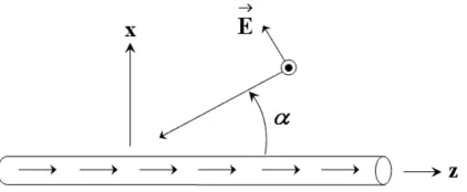
Now, we solve the problem of determining the scattered electromag-netic fields from a thin wire in free space. In Fig. 1, an electromagelectromag-netic wave traveling from the right encounters a wire at angleα.
Figure 1. An electromagnetic wave encounters a wire of radiusaand lengthLat an angle α.
According to boundary condition on the conductive surface:
Einc+Escat= 0 (14)
An expression is required to relate the current induced on a wire by an incident electric field to the scattered field it produces. For a wire along z-axis with a radius aof lengthL, the relationship is [28, 29]:
d2A(z)
dz2 +k
2A(z) =j4πω
0Ez(z) (15)
A(z) = L/2
−L/2
Iz(z)G(z, z)dz (16)
G(z, z) = 2π
0
e−jkR
R dφ
R= (z−z)2+
2asinφ 2
2
(18)
-0.25 -0. 2 -0.15 -0.1 -0.05 0 0.05 0.1 0.15 0.2 0.25 -2
1 0 1 2 3 4
Distance along wire (in terms of wave length)
Current (mA)
Magnitude Real
Imaginary
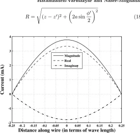
-Figure 2. Current distribution along the thin wire of length 12λ for
α= π2.
In many applications, the wire radius is very small compared with a wavelength. So, R is often approximated using the following form:
R≈(z−z)2+a2 (19)
The incident electric field along the conductor from a plane wave at angle α is:
Ez =ejkcosαsinα (20)
Consider a special case of a plane wave at broadside (α = π2). This plane wave will drive the current in a symmetrical manner. This implies that I(z) = I(−z), which means A(z) = A(−z). For these conditions, the final form of the integral equation of the wire current is [28]:
L/2
−L/2
Iz(z)G(z, z)dz =C1coskz+j 4πω0
k2sinαe
-0.5 -0.4 -0.3 -0.2 -0.1 0 0.1 0.2 0.3 0.4 0.5 -1
-0.8 -0.6 -0.4 -0.2 0 0.2 0.4 0.6 0.8 1
Distance along wire (in terms of wave length)
Current (mA)
Magnitude Real Imaginary
Figure 3. Current distribution along the thin wire of length λ for
α= π2.
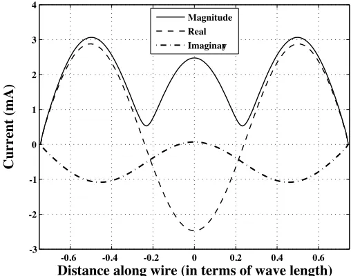
-0.6 -0.4 -0.2 0 0.2 0.4 0.6
-3 -2 -1 0 1 2 3 4
Distance along wire (in terms of wave length)
Current (mA)
Magnitude Real
Imaginary
Figure 4. Current distribution along the thin wire of length 32λ for
-1 -0.8 -0.6 -0.4 -0.2 0 0.2 0.4 0.6 0.8 1 -1.5
-1 -0.5 0 0.5 1 1.5
Distance along wire (in terms of wave length)
Current (mA)
Magnitude Real Imaginary
Figure 5. Current distribution along the thin wire of length 2λ for
α= π2.
0 20 40 60 80 100 120 140 160 180
-100 -95 -90 -85 -80 -75 -70 -65 -60 -55
Observation angle (degrees)
Radiation pattern (dB)
0 20 40 60 80 100 120 140 160 180 -95
-90 -85 -80 -75 -70 -65 -60 -55 -50
Observation angle (degrees)
Radiation pattern (dB)
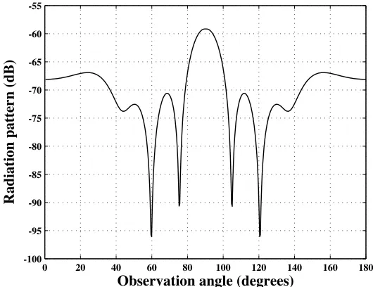
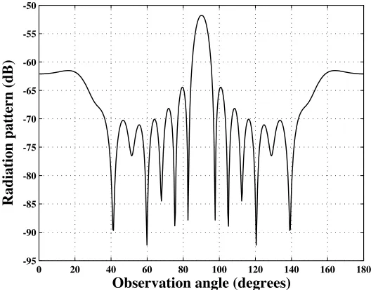
Figure 7. Radiation pattern of the thin wire of length 4λ.
This is a Fredholm integral equation of the first kind andC1 is an unknown coefficient that must be determined. For determiningC1, the number of match points must bem+ 1 instead ofm. The approximate solution of this equation gives the current distribution along the wire. Considering a= 0.001L, the current distributions for L= 12λ, λ, 32λ
and 2λ, and for α= π2 are shown in Figs. 2–5 respectively.
The radiation pattern of this wire is obtained of the following equation [30]:
f(α) = L/2
−L/2
Iz(z)ejkz
cosα
dz (22)
Also, it is possible to define a logarithmic quantity with respect tof, so that:
F = 20 log10|f| (dB) (23)
Figures 6 and 7 give the radiation patternF for L = 2λ and 4λ
5. CONCLUSION
The presented method in this paper is applied to solve the problem of determining the scattered electromagnetic fields from thin wires.
As the numerical results showed, this method reduces an integral equation of the first kind that is generally ill-posed to a well-condition linear system of algebraic equations.
The problem of determining the scattered fields was treated in detail. The presented approach can be generalized to apply to objects of arbitrary geometry.
REFERENCES
1. Mishra, M. and N. Gupta, “Monte Carlo integration technique for the analysis of electromagnetic scattering from conducting surfaces,” Progress In Electromagnetics Research, PIER 79, 91– 106, 2008.
2. Arnold, M. D., “An efficient solution for scattering by a perfectly conducting strip grating,”Journal of Electromagnetic Waves and Applications, Vol. 20, No. 7, 891–900, 2006.
3. Zhao, J. X., “Numerical and analytical formulations of the extended MIE theory for solving the sphere scattering problem,”
Journal of Electromagnetic Waves and Applications, Vol. 20,
No. 7, 967–983, 2006.
4. Ruppin, R., “Scattering of electromagnetic radiation by a perfect electromagnetic conductor sphere,” Journal of Electromagnetic Waves and Applications, Vol. 20, No. 12, 1569–1576, 2006. 5. Ruppin, R., “Scattering of electromagnetic radiation by a perfect
electromagnetic conductor cylinder,” Journal of Electromagnetic Waves and Applications, Vol. 20, No. 13, 1853–1860, 2006. 6. Hussein, K. F. A., “Efficient near-field computation for radiation
and scattering from conducting surfaces of arbitrary shape,”
Progress In Electromagnetics Research, PIER 69, 267–285, 2007. 7. Hussein, K. F. A., “Fast computational algorithm for EFIE
applied to arbitrarily-shaped conducting surfaces,” Progress In Electromagnetics Research, PIER 68, 339–357, 2007.
8. Kishk, A. A., “Electromagnetic scattering from composite objects using a mixture of exact and impedance boundary conditions,”
IEEE Transactions on Antennas and Propagation, Vol. 39, No. 6, 826–833, 1991.
nonlinear bounded dielectrics,”IEEE Transactions on Microwave Theory and Techniques, Vol. 43, No. 2, 428–436, 1995.
10. Shore, R. A. and A. D. Yaghjian, “Dual-surface integral equations in electromagnetic scattering,” IEEE Transactions on Antennas and Propagation, Vol. 53, No. 5, 1706–1709, 2005.
11. Yl¨a-Oijala, P. and M. Taskinen, “Well-conditioned M¨uller formulation for electromagnetic scattering by dielectric objects,”
IEEE Transactions on Antennas and Propagation, Vol. 53, No. 10, 3316–3323, 2005.
12. Li, L. W., P. S. Kooi, Y. L. Qin, T. S. Yeo, and M. S. Leong, “Analysis of electromagnetic scattering of conducting circular disk using a hybrid method,” Progress In Electromagnetics Research, PIER 20, 101–123, 1998.
13. Liu, Y. and K. J. Webb, “On detection of the interior resonance errors of surface integral boundary conditions for electromagnetic scattering problems,” IEEE Transactions on Antennas and Propagation, Vol. 49, No. 6, 939–943, 2001.
14. Kishk, A. A., “Electromagnetic scattering from transversely corrugated cylindrical structures using the asymptotic corrugated boundary conditions,” IEEE Transactions on Antennas and Propagation, Vol. 52, No. 11, 3104–3108, 2004.
15. Tong, M. S. and W. C. Chew, “Nystrom method with edge condition for electromagnetic scattering by 2d open structures,”
Progress In Electromagnetics Research, PIER 62, 49–68, 2006. 16. Valagiannopoulos, C. A., “Closed-form solution to the scattering
of a skew strip field by metallic pin in a slab,” Progress In Electromagnetics Research, PIER 79, 1–21, 2008.
17. Frangos, P. V. and D. L. Jaggard, “Analytical and numerical solution to the two-potential Zakharov-Shabat inverse scattering problem,” IEEE Transactions on Antennas and Propagation, Vol. 40, No. 4, 399–404, 1992.
18. Barkeshli, K. and J. L. Volakis, “Electromagnetic scattering from thin strips-Part II: Numerical solution for strips of arbitrary size,”
IEEE Transactions on Education, Vol. 47, No. 1, 107–113, 2004. 19. Collino, F., F. Millot, and S. Pernet, “Boundary-integral
methods for iterative solution of scattering problems with variable impedance surface condition,” Progress In Electromagnetics Research, PIER 80, 1–28, 2008.
20. Zahedi, M. M. and M. S. Abrishamian, “Scattering from semi-elliptic channel loaded with impedance elliptical cylinder,”
21. Zaki, K. A. and A. R. Neureuther, “Scattering from a perfectly conducting surface with a sinusoidal height profile: TE polarization,”IEEE Transactions on Antennas and Propagation, Vol. AP-19, No. 2, 208–214, 1971.
22. Carpentiery, B., “Fast iterative solution methods in electro-magnetic scattering,” Progress In Electromagnetics Research, PIER 79, 151–178, 2008.
23. Du, Y., Y. L. Luo, W. Z. Yan, and J. A. Kong, “An electromagnetic scattering model for soybean canopy,” Progress In Electromagnetics Research, PIER 79, 209–223, 2008.
24. Umashankar, K. R., S. Nimmagadda, and A. Taflove, “Numerical analysis of electromagnetic scattering by electrically large objects using spatial decomposition technique,” IEEE Transactions on Antennas and Propagation, Vol. 40, No. 8, 867–877, 1992.
25. Gokten, M., A. Z. Elsherbeni, and E. Arvas, “Electromagnetic scattering analysis using the two-dimensional MRFD formula-tion,”Progress In Electromagnetics Research, PIER 79, 387–399, 2008.
26. Delves, L. M. and J. L. Mohamed, Computational Methods for Integral Equations, Cambridge University Press, Cambridge, 1985. 27. Deb, A., A. Dasgupta, and G. Sarkar, “A new set of orthogonal functions and its application to the analysis of dynamic systems,”
Journal of the Franklin Institute, Vol. 343, 1–26, 2006.
28. Bancroft, R.,Understanding Electromagnetic Scattering Using the
Moment Method, Artech House, London, 1996.
29. Elliot, R. S., Antenna Theory and Design, Prentice Hall, Englewood Cliffs, New Jersey, 1981.