Tools for Simulating Features of Composite Order
Bilinear Groups in the Prime Order Setting
Allison Lewko ∗
The University of Texas at Austin
Abstract
In this paper, we explore a general methodology for converting composite order pairing-based cryptosystems into the prime order setting. We employ the dual pairing vector space approach initiated by Okamoto and Takashima and formulate versatile tools in this frame-work that can be used to translate composite order schemes for which the prior techniques of Freeman were insufficient. Our techniques are typically applicable for composite order schemes relying on the canceling property and proven secure from variants of the subgroup decision assumption, and will result in prime order schemes that are proven secure from the decisional linear assumption. As an instructive example, we obtain a translation of the Lewko-Waters composite order IBE scheme. This provides a close analog of the Boneh-Boyen IBE scheme that is proven fully secure from the decisional linear assumption. We also provide a translation of the Lewko-Waters unbounded HIBE scheme.
1
Introduction
Recently, several cryptosystems have been constructed in composite order bilinear groups and proven secure from instances (and close variants) of the general subgroup decision assump-tion defined in [3]. For example, the systems presented in [27, 25, 29, 28, 26] provide diverse and advanced functionalities like identity-based encryption (IBE), hierarchical identity-based encryption (HIBE), and attribute-based encryption with strong security guarantees (e.g. full security, leakage-resilience) proven from static assumptions. These works leverage convenient features of composite order bilinear groups that are not shared by prime order bilinear groups, most notably the presence of orthogonal subgroups of coprime orders. Up to isomorphism, a composite order bilinear group has the structure of a direct product of prime order subgroups, so every group element can be decomposed as the product of components in the separate sub-groups. However, when the group order is hard to factor, such a decomposition is hard to compute. The orthogonality of these subgroups means that they can function as independent spaces, allowing a system designer to use them in different ways without any cross interactions between them destroying correctness. Security relies on the assumption that these subgroups are essentially inseparable: given a random group element, it should be hard to decide which subgroups contribute non-trivial components to it.
Though composite order bilinear groups have appealing features, it is desirable to obtain the same functionalities and strong guarantees achieved in composite order groups from other assumptions, particularly from the decisional linear assumption (DLIN) in prime order bilinear groups. The ability to work with prime order bilinear groups instead of composite order ones
offers several advantages. First, we can obtain security under the more standard decisional linear assumption. Second, we can achieve much more efficient systems for the same security levels. This is because in composite order groups, security typically relies on the hardness of factoring the group order. This requires the use of large group orders, which results in considerably slower pairing operations.
There have been many previous examples of cryptosystems that were first built in composite order groups while later analogs were obtained in prime order groups. These include Groth-Ostrovsky-Sahai proofs [22, 21], the Boneh-Sahai-Waters traitor tracing scheme [10, 15], and the functional encryption schemes of Lewko-Okamoto-Sahai-Takashima-Waters [25, 33]. Waters also notes that the dual system encryption techniques in [39] used to obtain prime order systems were first instantiated in composite order groups. These results already suggest that there are strong parallels between the composite order and prime order settings, but the translation techniques are developed in system-specific ways.
Beyond improving the assumptions and efficiency for particular schemes, our goal in this paper is to expand our general understanding of how tools that are conveniently inherent in the composite order setting can be simulated in the prime order setting. We begin by asking: what are the basic features of composite order bilinear groups that are typically exploited by cryptographic constructions and security proofs? Freeman considers this question in [14] and identifies two such features, called projecting and canceling. These properties are defined in Section 2.3 below. Freeman then provides examples of how to construct either of these properties using pairings of vectors of group elements in prime order groups. Notably, Freeman does not provide a way of simultaneously achieving both projecting and canceling. There may be good reason for this, since Meiklejohn, Shacham, and Freeman [30] have shown that both properties cannot be simultaneously achieved in prime order groups when one relies on the decisional linear assumption in a “natural way”.
By instantiating either projecting or canceling in prime order groups, Freeman [14] suc-cessfully translates several composite order schemes into prime order schemes: the Boneh-Goh-Nissim encryption scheme [9], the Boneh-Sahai-Waters traitor tracing system [10], and the Katz-Sahai-Waters predicate encryption scheme [24]. These translations are accomplished using a three step process. The first step is to write the scheme in an abstract framework (replacing subgroups by subspaces of vectors in the exponent), the second step is to translate the assumptions into prime order analogs, and the third step is to transfer the security proof.
There are two aspects of Freeman’s approach that can render the results unsatisfying in certain cases. First, the step of translating the assumptions often does not result in standard assumptions like DLIN. A reduction to DLIN is only provided for the most basic variant of the subgroup decision assumption, and does not extend (for example) to the general subgroup decision assumption from [3]. Second, the step of translating the proof fails for many schemes, including all of the recent composite order schemes employing the dual system encryption proof methodology [27, 25, 29, 28, 26]. These schemes use only canceling and not projecting, and so this is unrelated to the limitations discussed in [30].
The reason for this failure is instructive to examine. As Freeman points out, “the recent identity-based encryption scheme of Lewko and Waters [27] uses explicitly in its security proof the fact that the groupGhas two subgroups of relatively prime order”. The major obstacle here is not translating the description of the scheme or its assumptions - instead the problem lies in translating a trick in the security proof. The trick works as follows. Suppose we have a group
G of order N =p1p2. . . pm, where p1, . . . , pm are distinct primes. Then if we take an element
g1∈Gof orderp1 (i.e. an element of the subgroup ofGwith orderp1) and a random exponent
even conditioned on amodp1 follows from the Chinese Remainder Theorem. In the security
proof of the Lewko-Waters scheme, there are elements of the formga
1 in the public parameters,
and the fact thatamodp2 remains information-theoretically hidden is later used to argue that all the keys and ciphertext received by the attacker are properly distributed in the midst of a hybrid argument.
Clearly, in a prime order group, we cannot hope to construct subgroups with coprime or-ders. There are a few possible paths for resolving this difficulty. We could start by reworking proofs in the composite order setting to avoid using this trick and then hope to apply the techniques of [14] without modification. This approach is likely to result in more complicated (though still static) assumptions in the composite order setting, which will translate into more complicated assumptions in the prime order setting. Since we prefer to rely only on the de-cisional linear assumption, we follow an alternate strategy: finding a version of this trick in prime order groups that does not rely on coprimeness. This is possible because coprimeness here is used a mechanism for achieving “parameter hiding,” meaning that some useful infor-mation is inforinfor-mation-theoretically hidden from the attacker, even after the public parameters are revealed. We can construct an alternate mechanism in prime order groups that similarly enables a form of parameter hiding.
Our Contribution We present versatile tools that can be used to translate composite or-der bilinear systems relying on canceling to prime oror-der bilinear systems, particularly those whose security proofs rely on general subgroup decision assumptions and employ the coprime mechanism discussed above. This includes schemes like [27], which could not be handled by Freeman’s methods. Our tools are based in the dual pairing vector space framework initiated by Okamoto and Takashima [31, 32]. We observe that dual pairing vector spaces provide a mech-anism for parameter hiding that can be used in place of coprimeness. We then formulate an assumption in prime order groups that can be used to mimic the effect of the general subgroup decision assumption in composite order groups. We prove that this assumption is implied by DLIN. Putting these ingredients together, we obtain a flexible toolkit for turning a new class of composite order constructions into prime order constructions that can be proven secure from DLIN.
We demonstrate the use of our toolkit by providing a translation of the composite order Lewko-Waters IBE construction [27]. This yields a prime order IBE construction that is proven fully secure from DLIN and also inherits the intuitive structure of the Boneh-Boyen IBE [5]. Compared to the fully secure prime order IBE construction in [39], our scheme achieves com-parable efficiency and security with a simpler structure. As a second application, we provide a translation of the Lewko-Waters unbounded HIBE scheme [29]. This additionally demonstrates how to handle delegation of secret keys with our tools.
1.1 Related Work
The concept of identity-based encryption was first proposed by Shamir [36] and later constructed by Boneh and Franklin [8] and Cocks [13]. In an identity-based encryption scheme, users are associated with identities and obtain secret keys from a master authority. Encryption to any identity can be done knowing only the identity and some global public parameters. Both of the initial constructions of IBE were proven secure in the random oracle model. The first standard model constructions, by Canetti, Halevi, and Katz [11] and Boneh and Boyen [5] relied on selective security, which is a more restrictive security model requiring the attacker to announce the identity to be attacker prior to viewing the public parameters. Subsequently, Boneh and Boyen [6], Gentry [16], and Waters [38, 39] provided constructions proven fully secure in the standard model from various assumptions. Except for the scheme of [13], which relied on the quadratic residuousity assumption, all of the schemes we have cited above rely on bilinear groups. A lattice-based IBE construction was first provided by Gentry, Peikert, and Vaikuntanathan in [18].
Hierarchical identity-based encryption was proposed by Horwitz and Lynn [23] and then constructed by Gentry and Silverberg [19] in the random oracle model. In a HIBE scheme, users are associated with identity vectors that indicate their places in a hierarchy (a user Alice is a superior of the user Bob if her identity vector is a prefix of his). Any user can obtain a secret key for his identity vector either from the master authority or from one of his superiors (i.e. a mechanism for key delegation to subordinates is provided). Selectively secure standard model constructions of HIBE were provided by Boneh and Boyen [5] and Boneh, Boyen, and Goh [7] in the bilinear setting and by Cash, Hofheinz, Kiltz, and Peikert [12] and Agrawal, Boneh, and Boyen [1, 2] in the lattice-based setting. Fully secure constructions allowing polynomial depth were given by Gentry and Halevi [17], Waters [39], and Lewko and Waters [27]. The first unbounded construction (meaning that the maximal depth is not bounded by the public parameters) was given by Lewko and Waters in [29].
Attribute-based encryption (ABE) is a more flexible functionality than (H)IBE, first intro-duced by Sahai and Waters in [35]. In an ABE scheme, keys and ciphertexts are associated with attributes and access policies instead of identities. In a ciphertext-policy ABE scheme, keys are associated with attributes and ciphertexts are associated with access policies. In a key-policy ABE scheme, keys are associated with access policies and ciphertexts are associ-ated with attributes. In both cases, a key can decrypt a ciphertext if and only if the at-tributes satisfy the formula. There are several constructions of both kinds of ABE schemes, e.g. [35, 20, 34, 4, 25, 33, 40].
The dual system encryption methodology was introduced by Waters in [39] as a tool for prov-ing full security of advanced functionalities such as (H)IBE and ABE. It was further developed in several subsequent works [27, 25, 33, 26, 29, 28]. Most of these works have used composite order groups as a convenient setting for instantiating the dual system methodology, with the exception of [33]. Here, we extend and generalize the techniques of [33] to demonstrate that this use of composite order groups can be viewed as an intermediary step in the development of prime order systems whose security relies on the DLIN assumption.
1.2 Organization
variant of the original Boneh-Boyen IBE scheme [5] that is proven fully secure from the decisional linear assumption. In Section 5, we briefly discuss how our techniques can be easily extended to schemes providing delegation capabilities, specifically the Lewko-Waters unbounded HIBE scheme in [29]. In Section 6, we discuss further extensions of our techniques. In Appendix A, we provide the formal definitions for IBE and HIBE and their standard IND-CPA security definitions. Finally, in Appendix B, we give the complete details of our prime order translation of the Lewko-Waters unbounded HIBE scheme and the proof of its security. We advise the reader that Appendix B is included for completeness, but is not necessary to understanding the main ideas of our work.
2
Background
2.1 Composite Order Bilinear Groups
WhenGis a bilinear group of composite orderN =p1p2. . . pm(wherep1, p2, . . . , pmare distinct
primes), we lete:G×G→GT denote its bilinear map (also referred to as a pairing). We note
that both G and GT are cyclic groups of order N. For each pi, G has a subgroup of order pi
denoted by Gpi. We let g1, . . . , gm denote generators of Gp1 through Gpm respectively. Each element g∈Gcan be expressed asg =ga1
1 g
a2
2 · · ·gamm for somea1, . . . , am ∈ZN, where eachai
is unique modulo pi. We will refer to giai as the “Gpi component” of g. When ai is congruent to zero modulo pi, we say that g has no Gpi component. The subgroups Gp1, . . . , Gpm are “orthogonal” under the bilinear map e, meaning that if h ∈ Gpi and u ∈ Gpj for i ̸=j, then
e(h, u) = 1, where 1 denotes the identity element in GT.
General Subgroup Decision Assumption The general subgroup decision assumption for composite order bilinear groups (formulated in [3]) is a family of static complexity assumptions based on the intuition that it should be hard to determine which components are present in a random group element, except for what can be trivially determined by testing for orthogonality with other given group elements. More precisely, for each non-empty subset S ⊆ [m], there is an associated subgroup of order ∏i∈Spi in G, which we will denote by GS. For two distinct,
non-empty subsets S0 and S1, we assume it is hard to distinguish a random element of GS0
from a random element ofGS1, when one is only given random elements of GS2, . . . , GSk where for each 2≤j≤k, either Sj∩S0=∅=Sj∩S1 orSj∩S0̸=∅ ̸=Sj∩S1.
More formally, we let G denote a group generation algorithm, which takes in m and a security parameter λand outputs a bilinear group G of order N =p1· · ·pm, where p1, . . . , pm
are distinct primes. The General Subgroup Decision Assumption with respect to G is defined as follows.
Definition 1. General Subgroup Decision Assumption. Let S0, S1, S2, . . . , Sk be non-empty subsets of[m]such that for each2≤j≤k, eitherSj∩S0 =∅=Sj∩S1 orSj∩S0̸=∅ ̸=Sj∩S1.
Given a group generator G, we define the following distribution:
G:= (N =p1· · ·pm, G, GT, e) R
←− G,
Z0
R
←−GS0, Z1 R
←−GS1, Z2 R
←−GS2, . . . , Zk R
←−GSk,
D:= (G, Z2, . . . , Zk).
We assume that for any PPT algorithm A (with output in {0,1}),
We note that this assumption holds in the generic group model, assuming it is hard to find a non-trivial factor of the group orderN.
Restricting to challenge sets differing by one element We observe that it suffices to consider challenge setsS0 andS1 of the formS1 =S0∪ {i}for somei∈[m],i /∈S0. We refer to this restricted class of subgroup decision assumptions as the 1-General Subgroup Decision As-sumption. To see that the 1-general subgroup decision assumption implies the general subgroup decision assumption, we show that any instance of the general subgroup decision assumption is implied by a sequence of the more restricted instances. More precisely, for general S0, S1, we
let U denote the set S0∪S1−S0. For anyiinU, the 1-general subgroup decision assumption implies that it hard to distinguish a random element ofGS0 from a random element ofGS0∪{i},
even given random elements from GS2, . . . , GSk. That is because each of the sets S2, . . . , Sk either does not intersectS1 orS0 and hence does not intersect S0 orS0∪ {i} ⊆S1, or intersects both S0 and S0∪ {i}. We can now incrementally add the other elements ofU using instances of the 1-general subgroup decision assumption, ultimately showing that it is hard to distin-guish a random element ofGS0 from a random element of GS0∪S1. We can reverse the process
and subtract one element at a time from S0∪S1 until we arrive at S1. Thus, the seemingly more restrictive 1-general subgroup decision assumption implies the general subgroup decision assumption.
2.2 Prime Order Bilinear Groups
We now let G denote a bilinear group of prime order p, with bilinear map e: G×G → GT.
More generally, one may have a bilinear map e: G×H → GT, where G and H are different
groups. For simplicity in this paper, we will always consider groups whereG=H.
In addition to referring to individual elements of G, we will also consider “vectors” of group elements. For⃗v= (v1, . . . , vn)∈Zpn and g∈G, we write g⃗v to denote a n-tuple of elements of
G:
g⃗v := (gv1, gv2, . . . , gvn).
We can also perform scalar multiplication and vector addition in the exponent. For anya∈Zp
and⃗v, ⃗w∈Znp, we have:
ga⃗v := (gav1, . . . , gavn), g⃗v+w⃗ = (gv1+w1, . . . , gvn+wn).
We defineen to denote the product of the componentwise pairings:
en(g⃗v, gw⃗) := n ∏
i=1
e(gvi, gwi) =e(g, g)⃗v·w⃗.
Here, the dot product is taken modulo p.
Dual Pairing Vector Spaces We will employ the concept of dual pairing vector spaces from [31, 32]. For a fixed (constant) dimensionn, we will choose two random bases B:= (⃗b1, . . . ,⃗bn)
and B∗ := (⃗b∗1, . . . ,⃗b∗n) of Znp, subject to the constraint that they are “dual orthonormal”, meaning that
whenever i̸=j, and
⃗bi·⃗b∗i =ψ
for alli, whereψis a uniformly random element ofZp. (This is a slight abuse of the terminology “orthonormal”, since ψis not constrained to be 1.)
For a generator g∈G, we note that
en(g⃗bi, g⃗b ∗
j) = 1
whenever i̸=j, where 1 here denotes the identity element in GT.
We note that choosing random dual orthonormal bases (B,B∗) can equivalently be thought of as choosing a random basis B, choosing a random vector⃗b∗1 subject to the constraint that it is orthogonal to⃗b2, . . . ,⃗bn, defining ψ=⃗b1·⃗b∗1, and then choosing⃗b∗2 so that it is orthogonal to ⃗b1,⃗b3, . . . ,⃗bn, and has dot product with⃗b2 equal to ψ, and so on. We will later use the notation
(D,D∗) and d1⃗ , . . . , etc. to also denote dual orthonormal bases and their vectors (and even
F,F∗ and f⃗1, etc.). This is because we will sometimes be handling more than one pair of dual
orthonormal bases at a time, and we use different notation to avoid confusing them.
Decisional Linear Assumption The complexity assumption we will rely on in prime order bilinear groups is the Decisional Linear Assumption. To define this formally, we letG denote a group generation algorithm, which takes in a security parameterλand outputs a bilinear group
Gof order p.
Definition 2. Decisional Linear Assumption. Given a group generator G, we define the fol-lowing distribution:
G:= (p, G, GT, e) R
←− G,
g, f, v, w←−R G, c1, c2, w
R
←−Zp, D:= (g, f, v, fc1, vc2).
We assume that for any PPT algorithm A (with output in {0,1}),
AdvG,A :=P [
A(D, gc1+c2) = 1]−P[A(D, gc1+c2+w) = 1]
is negligible in the security parameter λ.
2.3 Previously Investigated Abstract Properties of Bilinear Groups
We now define the abstract properties of projecting and canceling as formulated by Freeman [14]:
Projecting bilinear maps We say a bilinear map e : G×H → GT is projecting if there
exist subgroupsG1 ⊂G, H1 ⊂H, G′T ⊂Gand group homomorphisms π1,π2, and πT mapping
G, H, GT into themselves (respectively) such that G1 is the kernel ofπ1,H1 is the kernel of π2,
G′T is the kernel of πT, and these “projection maps” π1, π2, πT commute with e in the sense
that:
This structure is naturally achieved when the groups G, H, GT are of composite order N =
p1· · ·pm (where p1, . . . , pm are distinct primes), since we may take G1, H1, and G′T to be
the subgroups of order p1 inside G, H, GT respectively, and define the projections π1, π2 to be
exponentiation byp1 while πT is exponentiation by p21.
In this work, we will not consider projecting pairings and will instead be concerned with canceling pairings:
Canceling bilinear maps We say a bilinear map e : G×H → GT is canceling if there
are subgroups G1, . . . , Gm of G and H1, . . . , Hm of H such that G ∼= G1 ×. . .×Gm, H ∼=
H1×. . .×Hm, ande(gi, hj) = 1 in GT whenever gi ∈Gi, hj ∈Hj fori̸=j (here 1 represents
the identity element of GT). This structure is achieved naturally when the groups G, H, GT
are of composite order N =p1· · ·pm (where p1, . . . , pm are distinct primes), since we may set
Gi =Gpi, Hi =Hpi to be the subgroups of order pi for eachi. This structure is also achieved by dual orthonormal bases (B,B∗) in prime order groups, where each subgroupGi corresponds
to the span of vector⃗bi in the exponent, and each subgroup Hi corresponds to the span of the
vector⃗b∗i in the exponent. Here, the underlying bilinear mape:G×G→GT acts on two copies
of the same groupG, but we usedifferent bases in the exponents of our pairing en on n-tuples
of group elements.
3
Our Main Tools
There is an additional feature of composite order groups that is often exploited along with canceling in the security proofs for composite order constructions: we call thisparameter hiding. In composite order groups, parameter hiding takes the following form. Consider a composite order group G of orderN =p1p2 and an element g1 ∈Gp1 (an element of orderp1). Then if
we sample a uniformly random exponent a ∈ ZN and produce g1a, this reveals nothing about
the value ofamodulo p2. More precisely, the Chinese Remainder theorem guarantees that the value ofamodulop2 conditioned on the value ofamodulop1 is still uniformly random, andga1
only depends on the value ofamodulop1. This allows a party choosingato publishga1 and still
hide some information abouta, namely its value modulop2. Note that this party only needs to know N and g1: it does not need to know the factorization of N.
This is an extremely useful tool in security proofs, enabling a simulator to choose some secret random exponents, publish the public parameters by raising known subgroup elements to these exponents, and still information-theoretically hide the values of these exponents modulo some of the primes. These hidden values can be leveraged later in the security game to argue that something looks well-distributed in the attacker’s view, even if this does not hold in the simulator’s view. This sort of trick is crucial in proofs employing the dual system encryption methodology.
Replicating this trick in prime order groups seems challenging, since if one is given g and
3.1 Parameter Hiding in Dual Orthonormal Bases
We consider taking dual orthonormal bases and applying a linear change of basis to a subset of their vectors. We do this in such a way that we produce new dual orthonormal bases. In this subsection, we prove that if we start with randomly sampled dual orthonormal bases, then the resulting bases will also be random - in particular, the distribution of the final bases reveals nothing about the change of basis matrix that was employed. This “hidden” matrix can then be leveraged in security proofs as a way of separating the simulator’s view from the attacker’s. To describe this formally, we let m ≤ n be fixed positive integers and A ∈ Zmp×m be an invertible matrix. We let Sm⊆[n] be a subset of size m (|S|=m). For any dual orthonormal
bases B,B∗, we can then define new dual orthonormal bases BA,B∗A as follows. We let Bm
denote then×mmatrix over Zp whose columns are the vectors⃗bi ∈Bsuch thati∈Sm. Then
BmA is also an n×m matrix. We form BA by retaining all of the vectors⃗bi ∈ B for i /∈ Sm
and exchanging the⃗bi for i ∈ Sm with the columns of BmA. To define B∗A, we similarly let
Bm∗ denote the n×m matrix overZp whose columns are the vectors⃗b∗i ∈B∗ such that i∈Sm.
ThenBm∗(A−1)tis also an n×mmatrix, where (A−1)tdenotes the transpose of A−1. We form
B∗
Aby retaining all of the vectors⃗b∗i ∈B∗ fori /∈Sm and exchanging the⃗bi fori∈Sm with the
columns ofBm∗(A−1)t.
To see thatBAand B∗A are dual orthonormal bases, note that fori∈Sm, the corresponding
basis vector in BA can be expressed as a linear combination of the basis vectors⃗bj ∈ B with
j ∈ Sm, and the coefficients of this linear combination correspond to a column of A, say the
ℓth column (equivalently, say i is the ℓth element of Sm). When ℓ ̸= ℓ′, the ℓth column of A
is orthogonal to the (ℓ′)th column of (A−1)t. This means that the ith vector of BA will be
orthogonal to the (i′)th vector of B∗A whenever i̸=i′. Moreover, the ℓth column of A and the
ℓth column of (A−1)t have dot product equal to 1, so the dot product of the ith vector of BA and theith vector of B∗
A will be equal to the same value ψ as in the original basesBand B∗.
For a fixed dimensionn and primep, we let (B,B∗)←−R Dual(Zdp) denote choosing random dual orthonormal basesB and B∗ of Znp. Here, Dual(Znp) denotes the set of dual orthonormal bases.
Lemma 3. For any fixed positive integers m ≤ n, any fixed invertible A ∈ Zmp×m and set
Sm ⊆ [n] of size m, if (B,B∗) R
←− Dual(Zdp), then (BA,B∗A) is also distributed as a random sample from Dual(Zdp). In particular, the distribution of (BA,B∗A) is independent of A.
Proof. There is a one-to-one correspondence between (B,B∗) and (BA,B∗A): given (BA,B∗A), one can recover (B,B∗) by applyingA−1 to the vectors inBAwhose indices are inS
m, and applying
At to the corresponding vectors inB∗A. This shows that every pair of dual orthonormal bases is equally likely to occur as BA,B∗A.
3.2 Exploiting Hidden Parameters - An Example
We now give a small example of how a hidden change of basis matrix can be exploited by a simulator to hide a correlation from the attacker’s view. This example relies simply on pairwise independence of the functionf(x) =ax+bforx, a, b∈Zp whenaandbare chosen uniformly at random. Even this basic case is already quite useful - in particular, we will use this to establish full security for a close analog of the selectively secure Boneh-Boyen IBE scheme.
γA−1⃗z and λAt⃗y is negligibly close to the uniform distribution over Z2p ×Z2p. (Note that A is invertible with all but negligible probability.)
Proof. We let aij denote the i, j entry of A fori, j ∈ {1,2}. We may assume that A is
invert-ible, since this holds with overwhelming probability. Up to ignoring a scaling factor (which is irrelevant since our final vectors are randomly scaled by γ, λ), we can then write
A−1 =
(
a22 −a12
−a21 a11
)
, At=
(
a11 a21 a12 a22
)
.
We then have (still ignoring a scaling factor):
A−1⃗z=
(
a22−za12
−a21+za11
)
, At⃗y=
(
a11y−a21 a12y−a22
)
.
Since f(x) := a11x−a21 and g(x) := a12x−a22 are both pairwise independent functions of x,
and y̸=z, we have that these four entries are distributed as uniformly random inZ4
p.
Later, we will apply this lemma where y and zare distinct identities in an IBE scheme.
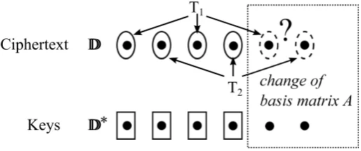
3.3 The Subspace Assumption
We now state a complexity assumption in prime order groups that we will use to simulate the effects of subgroup decision assumptions in composite order groups. We call this the Sub-space Assumption. We show that the subSub-space assumption is implied by the decisional linear assumption.
In prime order groups, basis vectors in the exponent take the place of subgroups. Since we are using dual orthonormal bases, our new concept of orthogonality between “subgroups” becomes asymmetric. If we have dual orthonormal basesB,B∗ and we think of “subgroup 1” in
Bas corresponding to the span of⃗b1, . . . ,⃗b4, then this is not orthogonal to the other vectors in
B, but it is orthogonal to vectors⃗b∗5, . . . ,⃗b∗n inB∗. Essentially, the notion of a single subgroup has now been split into a pair of “subgroups”, one for each side of the pairing, and orthogonality between different subgroups now only holds for elements on opposite sides.
This sort of asymmetry can be quite useful. For example, consider an instance of the general subgroup decision assumption in composite order groups, where the task is to distinguish a random element ofGp1 fromGp1p2. In this case, we cannot give out an element ofGp2, since it
can trivially be used to break the assumption by pairing it with the challenge term and seeing if the result is the identity. If we instead use dual orthonormal bases in a prime order group, the situation is a bit different. Suppose that given g⃗v, the task is to distinguish whether the exponent vector ⃗v is in the span of⃗b∗1,⃗b∗2 or in the larger span of⃗b∗1,⃗b∗2,⃗b∗3. We cannot give out g⃗b3, since one could then break the assumption by testing if e
n(g⃗v, g⃗b3) = e(g, g)⃗v·⃗b3 is the
identity, but we can give out gb⃗∗3.
Our definition of the subspace assumption is motivated by this and our observation in Section 2.1 that the general subgroup decision assumption in composite order groups can be restricted to distinguishing between sets that differ by one element. What this means is that to simulate the uses of the general subgroup decision in composite order groups, one can focus merely on creating an analog for expansion into one new “subgroup” at a time. At its core, our subspace assumption says that if one is given g⃗v, then it is hard to tell if ⃗v is randomly chosen from the span of⃗b∗1,⃗b∗2 or from the larger span of⃗b∗1,⃗b∗2,⃗b∗3, even if one is given scalar multiples of all bases vectors in Band B∗ in the exponent, except for⃗b3. We augment this by also given out a
the same structure for k 3-tuples of vectors, with the random linear combinations having the
same coefficients. (The fact that these coefficients are the same prevents this from following immediately from the assumption for a single 3-tuple applied in hybrid fashion.)
We now give the formal description of the subspace assumption. For a fixed dimensionn≥3 and prime p, we recall that (B,B∗)←−R Dual(Znp) denotes choosing random dual orthonormal basesBandB∗ ofZnp, andDual(Znp) denotes the set of dual orthonormal bases. Our assumption is additionally parameterized by a positive integerk≤ n3.
Definition 5. (Subspace Assumption) Given a group generator G, we define the following dis-tribution:
G:= (p, G, GT, e) R
←− G,
(B,B∗)←−R Dual(Znp),
g←−R G, η, β, τ1, τ2, τ3, µ1, µ2, µ3
R
←−Zp,
U1 :=gµ1⃗b1+µ2⃗bk+1+µ3⃗b2k+1, U2 :=gµ1⃗b2+µ2⃗bk+2+µ3⃗b2k+2, . . . , U
k:=gµ1⃗bk+µ2⃗b2k+µ3⃗b3k,
V1 :=gτ1η⃗b
∗
1+τ2β⃗b∗k+1, V
2:=gτ1η⃗b
∗
2+τ2β⃗b∗k+2, . . . , V
k :=gτ1η⃗b ∗
k+τ2β⃗b∗2k
W1 :=gτ1η⃗b∗1+τ2β⃗b∗k+1+τ3⃗b∗2k+1, W2:=gτ1η⃗b∗2+τ2β⃗b∗k+2+τ3⃗b∗2k+2, . . . , W
k:=gτ1η⃗b ∗
k+τ2β⃗b∗2k+τ3⃗b∗3k
D:=(g⃗b1, g⃗b2, . . . , g⃗b2k, g⃗b3k+1, . . . , g⃗bn, gη⃗b∗1, . . . , gη⃗b∗k, gβ⃗b∗k+1, . . . , gβ⃗b∗2k, g⃗b∗2k+1, . . . , g⃗b∗n, U
1, U2, . . . , Uk, µ3
)
.
We assume that for any PPT algorithm A (with output in {0,1}),
AdvG,A :=|P[A(D, V1, . . . , Vk) = 1]−P[A(D, W1, . . . , Wk) = 1]| is negligible in the security parameter λ.
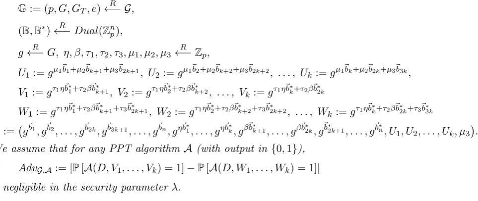
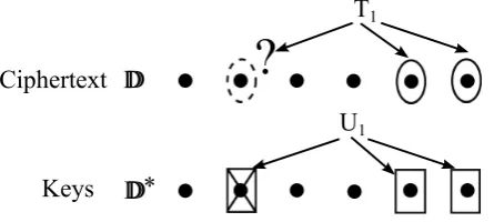
We have included in D more terms than will be necessary for many applications of this assumption, and in what follows we will often omit those we do not need. We will work exclusively with the k = 1 and k = 2 cases. We present the assumption in the form above in order make it more versatile for use in future applications. We additionally note that the form stated above can be further generalized to involve multiple, independently generated dual orthonormal bases (B1,B∗1),(B2,B∗2), . . . ,(Bj,B∗j), for any fixedj. The terms in the assumption
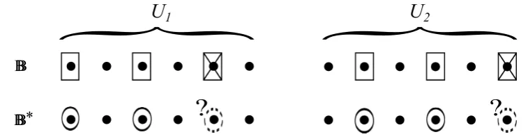
would be duplicated for each pair of bases, with the same values of η, β, τ1, τ2, τ3, µ1, µ2, µ3. We will not need this generalization for the applications we present. To help the reader see the main structure of this assumption through the burdensome notation, we include heuristic illustrations of thek= 1 andk= 2 cases below.
BB
BB*
?
U1
{
Figure 1: Subspace Assumption withk= 1
In these diagrams, the top rows illustrate the U terms, while the bottom rows illustrate the V, W terms. The solid ovals and rectangles indicate the presence of basis vectors. The crossed rectangles indicate basis elements of B which are present in U1, U2 but are not given
BB
BB*
?
?
{
U
1{
U
2Figure 2: Subspace Assumption withk= 2
3.4 Reduction to the Decisional Linear Assumption
We now show that our subspace assumption is implied by the decisional linear assumption.
Lemma 6. If the decisional linear assumption holds for a group generatorG, then the subspace assumption stated in Definition 5 also holds for G.
Proof. We assume there exists a PPT algorithmAbreaking the subspace assumption with non-negligible advantage (for some fixed positive integers k, n satisfying n≥3k). We will use this to create a PPT algorithmBwhich breaks the decisional linear assumption with non-negligible advantage. B is given g, f, v, fc1, vc2, T, where T is either gc1+c2 or T is a uniformly random
element of G. We let ℓf denote the discrete logarithm base g of f and ℓv denote the discrete
logarithm baseg of v, i.e. f =gℓf and v=gℓv.
B simulates the subspace assumption for A as follows. B first samples random dual or-thonormal bases, denoted by d1, . . . , ⃗⃗ dn and d⃗1∗, . . . , ⃗d∗n. In other words, B chooses vectors
⃗
d1, . . . , ⃗dn, ⃗d∗1, . . . , ⃗d∗nrandomly, subject to the constraints thatd⃗i·d⃗∗j ≡0 modpwheni̸=j, and
⃗
di·d⃗∗i ≡ψmodp for all i from 1 ton, where ψ is a random element ofZp. Now, B implicitly
sets:
η⃗b∗1=d⃗∗2k+1+ℓfd⃗∗1, η⃗b∗2=d⃗∗2k+2+ℓfd⃗∗2, . . . , η⃗b∗k=d⃗∗3k+ℓfd⃗∗k,
β⃗bk∗+1 =d⃗∗2k+1+ℓvd⃗∗k+1, β⃗b∗k+2 =d⃗∗2k+2+ℓvd⃗∗k+2, . . . , β⃗b∗2k=d⃗∗3k+ℓvd⃗∗2k,
⃗b∗
2k+1 =d⃗∗2k+1, . . . ,⃗b∗n=d⃗∗n.
We think of this as setting η=ℓf and β=ℓv, with⃗b∗1 =η−1d⃗∗2k+1+d⃗∗1 for example.
B sets the dual basis as:
⃗b1 =d⃗1, ⃗b2 =d⃗2, . . . ,⃗b2k=d⃗2k,
⃗b2k+1 =d⃗2k+1−ℓ−f1d1⃗ −ℓ−
1
v d⃗k+1, . . . , ⃗b3k=d⃗3k−ℓf−1d⃗k−ℓ−v1d⃗2k,
⃗b3k+1 =d⃗3k+1, . . . , ⃗bn=d⃗n.
We observe that under these definitions, ⃗bi·⃗b∗j ≡ 0 modp whenever i ̸= j, and ⃗bi ·⃗b∗i =
⃗
di·d⃗∗i =ψfor allifrom 1 ton. We note thatBcan produce all ofgη⃗b ∗
1, . . . , gη⃗b∗k,gβ⃗b∗k+1, . . . , gβ⃗b∗2k,
g⃗b∗2k+1, . . . , g⃗bn∗,g⃗b1, . . . , g⃗b2k, and g⃗b3k+1, . . . , g⃗bn, butcannot produce g⃗b2k+1, . . . , g⃗b3k.
We argue that η=ℓf,β=ℓv,⃗b1, . . . ,⃗bnand⃗b∗1, . . . ,⃗b∗nare properly distributed. To see this,
note that given any dual orthonormal bases⃗b1, . . . ,⃗bn and⃗b1∗, . . . ,⃗b∗n, and any η, β, one can
solve for a unique dual orthonormal bases d⃗1, . . . , ⃗dn and d⃗∗1, . . . , ⃗d∗n (with the same value ofψ)
which yields⃗b1, . . . ,⃗bn and⃗b∗1, . . . ,⃗b∗n via the equations above. Thus,η =ℓf,β =ℓv,⃗b1, . . . ,⃗bn
Now Bcreates U1, . . . , Uk as follows. It chooses random valuesµ1′, µ′2, µ′3 ∈Zp. It sets:
U1 =gµ
′
1⃗b1+µ′2⃗bk+1+µ′3d⃗2k+1.
We note that
µ′1⃗b1+µ′2⃗bk+1+µ3′d⃗2k+1= (µ′1+ℓ−f1µ′3)⃗b1+ (µ′2+ℓ−v1µ′3)⃗bk+1+µ′3⃗b2k+1.
In other words,B has implicitly set µ1 =µ′1+ℓ− 1
f µ′3, µ2 =µ′2+ℓv−1µ′3, and µ3 =µ′3. We note
that these values are uniformly random, and µ3 is known toB. Bcan then form U2, . . . , Uk as:
U2 =gµ
′
1⃗b2+µ′2⃗bk+2+µ′3d⃗2k+2, . . . , U k=gµ
′
1⃗bk+µ′2⃗b2k+µ′3d⃗3k.
B then implicitly sets τ1=c1 and τ2 =c2. We note that
τ1η⃗b∗1+τ2β⃗b∗k+1 = (c1+c2)d⃗∗2k+1+c1ℓfd⃗∗1+c2ℓvd⃗∗k+1,
.. .
τ1η⃗b∗k+τ2β⃗b∗2k = (c1+c2)d⃗3∗k+c1ℓfd⃗∗k+c2ℓvd⃗∗2k.
The terms which are multiples ofc1ℓf and c2ℓv are not difficult for B to produce as exponents
of g, sinceB hasfc1 =gc1ℓf and vc2 =gc2ℓv. For the multiples of c1+c2,B needs to use T.
B computes:
T1 =Td⃗∗2k+1(fc1)d⃗∗1(vc2)d⃗∗k+1, . . . , T k =T
⃗
d∗3k(fc1)d⃗k∗(vc2)d⃗∗2k.
If T = gc1+c2, then these are distributed as V1, . . . , V
k. If T = gc1+c2+w, then these are
dis-tributed as W1, . . . , Wk, withτ3 implicitly set to w.
B gives
D:=(g⃗b1, g⃗b2, . . . , g⃗b2k, g⃗b3k+1, . . . , g⃗bn, gη⃗b∗1, . . . , gη⃗b∗k, gβ⃗b∗k+1, . . . , gβ⃗b∗2k,
g⃗b∗2k+1, . . . , g⃗b∗n, U1, U2, . . . , U
k, µ3 )
toA, along withT1, . . . , Tk. Bcan then leverageA’s non-negligible advantage in distinguishing
between the distributions (V1, . . . , Vk) and (W1, . . . , Wk) to achieve a non-negligible advantage in
distinguishing T =gc1+c2 from T =gc1+c2+w, hence violating the decisional linear assumption.
We note that the above reduction can be parallelized for multiple bases (B1,B∗1), (B2,B∗2),. . .,
(Bj,B∗j) by having the simulator sample (D1,D∗1), . . . ,(Dj,D∗j) independently and follow the same procedure for each.
4
Analog of the Boneh-Boyen IBE Scheme
In this section, we employ our subspace assumption and our parameter hiding technique for dual orthonormal bases to prove full security for a close analog of the Boneh-Boyen IBE scheme from the decisional linear assumption. This is the same security guarantee achieved for the IBE scheme in [39] and our efficiency is also similar. The advantage of our scheme is that it is a much closer analog to the original Boneh-Boyen IBE, and resultingly has a simpler, more intuitive structure.
4.1 Review of the Boneh-Boyen Scheme
We begin by reviewing the original Boneh-Boyen scheme [5] in prime order bilinear groups, which was proven to be selectively secure. In this scheme, the public parameters consist of three random elements ofG and one element of GT:
PP :={g, u, h∈G, e(g, g)α}.
Here,α is random element of Zp, and MSK =gα. Identities are assumed to be elements ofZp, and a secret key for identityID is of the form
SKID={gα(uIDh)r, gr},
wherer is a random value inZp chosen by the master authority when it is called upon to issue this secret key. Messages are assumed to be elements of GT, and an encryption of a message
M to an identityID takes the form:
CT ={M e(g, g)αs, gs,(uIDh)s},
wheresis a random value in Zp chosen by the encryptor. Decryption works by computing two pairings and dividing the result to obtain:
e(gα(uIDh)r, gs)/e(gr,(uIDh)s) =e(g, g)αs,
which can then be divided from M e(g, g)αs to obtain M.
This scheme is quite elegant in its simplicity - every parameter plays a clear role. The ran-domnesssis used to randomize ciphertexts. The randomnessrembedded in a user’s secret key prevents the user from recovering the master secret key. The parameter h prevents multiplica-tive manipulations of identities: for example, suppose one user has identity ID and another has identity 2ID. If the parameter h were absent, the user with identity 2ID could take a ciphertext encrypted toIDand raise the last element to the power 2 to obtain a ciphertext for his identity 2ID. The parameter uprevents users from removing the dependence on identities. For example, if we used gID in place of uID, then a user could take the gr term in his secret key, raise it to the power ID, and use this to strip off the identity-dependent term from the first part of his key.
4.2 Review of the Lewko-Waters Composite Order Variant
The Lewko-Waters IBE scheme [27] takes the Boneh-Boyen IBE and embeds it into the first subgroup of a bilinear group of composite order N =p1p2p3. Random elements from Gp3 are
multiplied to key elements for additional randomization. This results in a scheme that retains the intuitive structure of Boneh-Boyen. In fact its description is almost identical, except that nowg, u, hare replaced by g1, u1, h1 ∈Gp1, and keys are of the form:
SKID={gα1(uID1 h1)rR3, g1rR′3},
whereR3, R′3 are randomly chosen elements of Gp3. Since the ciphertext elementsg s
1,(uID1 h1)s
are contained in Gp1, these extra terms R3, R′3 are orthogonal to the ciphertext and do not
hinder decryption.
in the proof. The relationships between these objects are as follows: normal keys can decrypt both normal and semi-functional ciphertexts, while semi-functional keys can only decrypt nor-mal ciphertexts. When a semi-functional key is used to decrypt a semi-functional ciphertext, decryption will fail with all but negligible probability.
The security proof for a dual system is accomplished via a hybrid argument argument over a sequence of games. The first game is the real security game with normal keys and a normal ciphertext. In the next game, the ciphertext given to the attacker is changed to be semi-functional. Then, the keys given to the attacker are changed to be semi-functional, one by one. Once everything the attacker receives is semi-functional, then it is typically easy to prove security directly.
Semi-functional keys and ciphertexts in the LW IBE are just like normal keys and ciphertexts in the subgroups Gp1 and Gp3, with additional random components in Gp2. More precisely, a
semi-functional ciphertext is of the form
CT ={M e(g1, g1)αs, g1sX2,(uID1 h1)sX2′},
whereX2, X2′ are random elements in Gp2. Similarly, a semi-functional key is of the form
SKID={gα1(uID1 h1)rR3Y2, gr1R3′Y2′},
where Y2, Y2′ are random elements in Gp2. Note that these elements in Gp2 affect decryption
only when a semi-functional key and a semi-functional ciphertext are paired together.
To execute the game transitions in the hybrid proof, one must argue that an attacker’s advantage cannot change noticeably between adjacent games. This is done by showing that if one is given a PPT attacker whose advantage noticeably changes, then one can create a PPT simulator which leverages this attacker to break a computational assumption. It is relatively straightforward to use a subgroup decision assumption to change the ciphertext from normal to semi-functional: the simulator will be given g1 ∈Gp1, g3 ∈ Gp3 and T, and its task will be
to decide if T ∈Gp1 or T ∈Gp1p2. It will setu1 =g a
1 and h1 =g1b, where it knowsa, b∈ZN,
and can then implicitly setgs1 to be theGp1 component ofT. It can compute the final element
of the ciphertext as TaID+b. If T ∈ Gp1, this is a properly distributed normal ciphertext. If
T ∈Gp1p2, this is a properly distributed semi-functional ciphertext (note that the values ofa, b
modulop2 are uniformly random, even conditioned on the public parameters, which only reveal their values modulo p1).
the identity of the challenge ciphertext. In the LW proof, this is accomplished via a pairwise independent function, f(ID) :=aID+b modulo p2. The value ofa modulo p1 is the discrete
log ofu1 baseg1, while the value of b modulop1 is the discrete log of h1 baseg1. Information-theoretically, the public parameters revealamodp1andbmodp1, but the values ofamodp2 and bmodp2 remain hidden. The pairwise independence of the function f modulo p2 can thus be
invoked to argue that the semi-functional components of the challenge ciphertext and challenge key appear properly distributed in the attacker’s view. For more details of this argument, see [27].
The subgroup decision assumption used for this step in the proof is as follows: given random elements in Gp1, Gp3, Gp1p2, and Gp2p3, it should be hard to distinguish a random element of
Gp1p3 from a random element ofG. The element ofGp1 is used to make the public parameters,
the element of Gp3 is used to randomize normal keys, the element of Gp1p2 is used to make
the semi-functional ciphertext, the element of Gp2p3 is used to make the semi-functional keys,
and the element of unknown type is used to make the challenge key (its Gp1 component is
implicitly set to be gr1). Because the Gp2 components of the challenge ciphertext and the
(possibly present)Gp2 components of the challenge key both enter via group elements that also
have Gp1 components, the exponents of these elements must conform to the structure of the
scheme that is enforced in the Gp1 subgroup - this is what causes nominal semi-functionality
when the identities are the same: the cancelation that happens in theGp1 subgroup is mirrored
in theGp2 subgroup. Essentially, what we get is a second copy of the scheme occurring in theGp2
subgroup for the challenge key and challenge ciphertext, but with “fresh” parametersamodp2
and bmodp2 that are not constrained by the public parameters. This hides the structure in
Gp2 via pairwise independence when the identities are unequal.
4.3 Our Construction
We now construct an analog of the Boneh-Boyen IBE scheme in prime order bilinear groups that can be proven fully secure by mimicking the LW proof strategy. We will use dual orthonormal bases (D,D∗) ofZ6p, wherepis the prime order of our bilinear group G. Public parameters and ciphertexts will have exponents described in terms of the basis vectors in D, while secret keys will have exponents described in terms ofD∗. The first four basis vectors of each will constitute the “normal space” (like Gp1 in the LW scheme), and the last two basis vectors of each will
constitute the “semi-functional space” (likeGp2 in the LW scheme).
By using dual pairing vector spaces, we avoid the need to simulateGp3. In the LW scheme,
the purpose of Gp3 is to allow the creation of other semi-functional keys while a challenge key
is changing from normal to semi-functional. More precisely, it allows the subgroup decision assumption to give out an element of Gp2p3 that can be used to generate semi-functional keys
when the task is to distinguish a random element ofGp1p3 from a random element ofG. We note
that if we did not useGp3 here and instead tried to create all of the semi-functional keys from a
term inGp1p2, then these keys would not be properly randomized in theGp2 subgroup because
the structure of the scheme is enforced in theGp1 subgroup. Pairwise independence cannot save
us here because there are many keys. However, the asymmetry of dual pairing vector spaces avoids this issue: while we are expanding the challenge key into the “semi-functional space” in
D∗, we can still know a basis for the semi-functional space ofD∗ in the exponent - it is only the
corresponding terms in the semi-functional space ofDthat we do not have access to in isolation. This allows us to make the other semi-functional keys without needing to create an analog of theGp3 subgroup.
the identity appearing on the key side. This is combined with a mechanism for preventing multiplication manipulation of the identity. In our scheme, this core cancelation is duplicated: instead of having one cancelation, we have two, each with its own random coefficients. The first cancelation will occur for the d⃗1, ⃗d2 and d⃗∗1, ⃗d∗2 components, and the second will occur for the
⃗
d3, ⃗d4 and d⃗∗3, ⃗d∗4 components.
This expansion gives us room to use the subspace assumption with parameter k = 2 to transition from 4-dimensional exponents for normal keys and ciphertexts to 6-dimensional ex-ponents for semi-functional keys and ciphertexts. Having a 2-dimensional semi-functional space allows us to implement nominal semi-functionality. We will elaborate on this below after defin-ing the semi-functional objects for our scheme. To prevent multiplicative manipulations of the identities in our scheme is rather easy, since the orthogonality of the dual bases allows us to “tie” all the components of the keys and ciphertexts together without causing cross interactions that interfere with decryption.
We assume that messagesM are elements ofGT (the target group of the bilinear map) and
that identitiesID are elements of Zp.
Setup(λ) →MSK,PP The setup algorithm takes in the security parameter λand chooses a bilinear groupGof sufficiently large prime order p. We lete:G×G→GT denote the bilinear
map. We set n = 6. The algorithm samples random dual orthonormal bases, (D,D∗) ←−R
Dual(Znp). We letd1, . . . , ⃗⃗ d6 denote the elements of Dand d⃗∗1, . . . , ⃗d∗6 denote the elements ofD∗. It also chooses random values α, θ, σ∈Zp. The public parameters are computed as:
PP :=
{
G, p, e(g, g)αθ ⃗d1·d⃗∗1, gd⃗1, . . . , gd⃗4 }
.
(We note thatd⃗1·d⃗1∗=ψby definition ofD,D∗, but we write out the dot product when we feel
it is more instructive.) The master secret key is:
MSK :=
{
gθ ⃗d∗1, gαθ ⃗d∗1, gθ ⃗d∗2, gσ ⃗d∗3, gσ ⃗d∗4 }
.
KeyGen(MSK, ID)→SKID The key generation algorithm chooses random valuesr1, r2∈Zp
and forms the secret key as:
SKID:=g(α+r1ID)θ ⃗d ∗
1−r1θ ⃗d∗2+r2IDσ ⃗d∗3−r2σ ⃗d∗4.
Encrypt(M, ID,PP)→CT The encryption algorithm chooses random valuess1, s2 ∈Zp and forms the ciphertext as:
CT :=
{
C1:=M
(
e(g, g)αθ ⃗d1·d⃗∗1 )s1
, C2 :=gs1d⃗1+s1ID ⃗d2+s2d⃗3+s2ID ⃗d4 }
.
Decrypt(CT,SKID)→M The decryption algorithm computes the message as:
M :=C1/en(SKID, C2).
4.4 Correctness
We observe that when the ciphertext is encrypted underID, then:
en(SKID, C2) =e(g, g)s1(α+r1ID)θ ⃗d1· ⃗
d∗1−s1IDr1θ ⃗d2·d⃗∗2+s2r2IDσ ⃗d3·d⃗∗3−s2IDr2σ ⃗d4·d⃗∗4.
Since d⃗1·d⃗∗1=d⃗2·d⃗∗2=d⃗3·d⃗∗3 =d⃗4·d⃗∗4 =ψ, this exponent is equal to:
(s1αθ+s1r1IDθ−s1r1IDθ+s2r2IDσ−s2r2IDσ)ψ=s1αθψ.
Noting that
C1=M e(g, g)s1αθψ,
correctness follows.
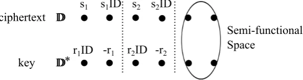
A visual representation of the structure of our construction is below in Figure 3. In our illustration, we leave out theαcontribution as well as theθandσ parameters in order to get an uncluttered look at the core structure of the cancelations that occur in our decryption algorithm. We indicate the semi-functional space to be the span of the vectors d⃗5, ⃗d6 for ciphertexts and
the span of the vectorsd⃗∗5, ⃗d∗6 for keys. Semi-functional ciphertexts and keys will include random vectors in these spaces. These are formally defined in the next subsection.
DD
* DD
Semi-functional Space
r1ID
s1
-r1
s1ID s2 s2ID
r2ID -r2
ciphertext
key
Figure 3: Cancelation in our construction
4.5 Semi-functional Algorithms
We choose to define our semi-functional objects by providing algorithms that generate them. We note that these algorithms are only provided for definitional purposes, and are not part of the IBE system. In particular, they do not need to be efficiently computable from the public parameters and master secret key alone.
KeyGenSF The semi-functional key generation algorithm chooses random valuesr1, r2, t5, t6 ∈
Zp and forms the secret key as
SKID:=g(α+r1ID)θ ⃗d ∗
1−r1θ ⃗d∗2+r2IDσ ⃗d∗3−r2σ ⃗d∗4+t5d⃗5∗+t6d⃗∗6.
This is distributed like a normal key with additional random multiples of d⃗∗5 and d⃗∗6 added in the exponent.
EncryptSF The semi-functional encryption algorithm chooses random values s1, s2, z5, z6 ∈
Zp and forms the ciphertext as:
CT :=
{
C1:=M
(
e(g, g)αθ ⃗d1·d⃗∗1 )s1
, C2 :=gs1
⃗
d1+s1ID ⃗d2+s2d⃗3+s2ID ⃗d4+z5d⃗5+z6d⃗6 }
This is distributed like a normal ciphertext with additional random multiples ofd⃗5 andd⃗6added
in the exponent.
We observe that if one applies the decryption procedure with a semi-functional key and a normal ciphertext, decryption will succeed because d⃗∗5, ⃗d∗6 are orthogonal to all of the vectors in exponent of C2, and hence have no effect on decryption. Similarly, decryption of a
semi-functional ciphertext by a normal key will also succeed because d5, ⃗⃗ d6 are orthogonal to all of the vectors in the exponent of the key. Whenboth the ciphertext and key are semi-functional, the result ofen(SKID, C2) will have an additional term, namely
e(g, g)t5z5d⃗5·d⃗∗5+t6z6d⃗6·d⃗∗6 =e(g, g)(t5z5+t6z6)ψ.
Decryption will then fail unless t5z5+t6z6 ≡0 modp. If this modular equation holds, we say that the key and ciphertext pair is nominally semi-functional. We note that this is possible, even when none of t5, z5, t6, z6 are congruent to zero modulop- this is why we have designated
a semi-functional space of dimension 2. Requiring the 1-dimensional version of this modular equation, i.e. t5z5≡0 modp, would be equivalent to requiring that eithert5 orz5 be congruent to zero modulop.
4.6 Proof of Security
We now prove the following theorem:
Theorem 7. Under the decisional linear assumption, the IBE scheme presented in Section 4.3 is fully secure.
We prove this using a hybrid argument over a sequence of games, following the LW strategy. We start with the real security game, denoted by Gamereal. We letqdenote the number of keys
requested by the attacker. We define the following additional games.
Gamei for i= 0,1, . . . , q Gamei is like Gamereal, except the ciphertext given to the attacker
is semi-functional (i.e. generated by a call to EncryptSF instead of Encrypt) and the first i
keys given to the attacker are semi-functional (generated by KeyGenSF). The remaining keys are normal. We note that in Game0, all of the keys are normal, and in Gameq, all of the keys
are semi-functional.
Gamef inal Gamef inalis like Gameq, except that the ciphertext is a semi-functional encryption
of arandom message inGT, instead of one of the messages supplied by the attacker.
We transition from Gamereal to Game0, then to Game1, and so on, until we arrive at
Gameq. We prove that with each transition, the attacker’s advantage cannot change by a
non-negligible amount. As a last step, we transition to Gamef inal, where it is clear that the attacker’s
advantage is zero. These transitions are accomplished in the following lemmas, all using the subspace assumption. We letAdvArealdenote the advantage of an algorithmAin the real game,
Advi
A denote its advantage in Gamei, and Advf inalA denote its advantage in Gamef inal.
We begin with the transition from Gamereal to Game0. At the analogous step in the LW
proof, a subgroup decision assumption is used to expand the ciphertext from Gp1 into Gp1p2.
Here, we use the subspace assumption with k = 2 to expand the ciphertext exponent vector from the span ofd1, . . . , ⃗⃗ d4into the larger span ofd1, . . . , ⃗⃗ d6. We use a very basic instance of the parameter hiding technique to argue that the resulting coefficients of d⃗5 and d⃗6 are randomly