Scholarship@Western
Scholarship@Western
Electronic Thesis and Dissertation Repository
7-27-2018 1:30 PM
The Statistical Exploration in the $G$-expectation Framework: The
The Statistical Exploration in the $G$-expectation Framework: The
Pseudo Simulation and Estimation of Variance Uncertainty
Pseudo Simulation and Estimation of Variance Uncertainty
Yifan Li
The University of Western Ontario
Supervisor Kulperger, Reg
The University of Western Ontario
Graduate Program in Statistics and Actuarial Sciences
A thesis submitted in partial fulfillment of the requirements for the degree in Master of Science © Yifan Li 2018
Follow this and additional works at: https://ir.lib.uwo.ca/etd Part of the Probability Commons
Recommended Citation Recommended Citation
Li, Yifan, "The Statistical Exploration in the $G$-expectation Framework: The Pseudo Simulation and Estimation of Variance Uncertainty" (2018). Electronic Thesis and Dissertation Repository. 5530. https://ir.lib.uwo.ca/etd/5530
This Dissertation/Thesis is brought to you for free and open access by Scholarship@Western. It has been accepted for inclusion in Electronic Thesis and Dissertation Repository by an authorized administrator of
TheG-expectation framework, motivated by problems withuncertainty, is a new generalization
of the classical probability framework. Similar to the Choquet expectation, the G-expectation
can be represented as the supremum of a class of linear expectations. In the past two decades, it has developed into a complete stochastic structure connected with a large family of nonlinear PDEs. Nonetheless, to apply it to real-world problems with uncertainty, it is fundamentally necessary to build up the associated statistical methodology.
This thesis explores the computation, simulation, and estimation of the G-normal
distri-bution (a typical distridistri-bution with variance uncertainty) by constructing a new substructure called the Semi-G-normal distributionwhich provides the transition from classical normal to
G-normal distribution. Interestingly, it also gives an efficient iterative scheme to stochastically
solve the nonlinearBlack-Scholes-Barenblatt equation with volatility uncertainty. This thesis is
the theoretical and technical preparation for the future industrial application ofG-framework.
Keywords:Uncertainty,G-expectation framework, Semi-G-normal distribution, Sublinear
expectation, Statistical theory, Black-Scholes-Barenblatt equation
Abstract i
List of Figures iv
List of Tables v
1 Introduction 1
1.1 Background of theG-framework . . . 1
1.1.1 A simple story: What isUncertainty? . . . 2
1.1.2 Literature review: How do we deal withUncertainty? . . . 6
1.2 Overview of my research . . . 9
2 The Distributions and Independence in theG-framework 12 2.1 Preliminaries . . . 12
2.2 Motivation: How can we better understand theG-normal distribution? . . . 18
2.3 The semi-G-normal distribution andG-normal distribution . . . 19
2.3.1 The 1-dimensional situation . . . 19
2.3.2 Thed-dimensional situation . . . 31
2.3.3 Implementation . . . 32
The 1-dimensional case . . . 32
Thed-dimensional case . . . 35
2.3.4 Assessment of the iterative method and future exploration . . . 37
2.4 The sequential independence in theG-framework . . . 39
2.4.1 Independence regardingG-normal distributions . . . 40
2.4.2 Independence regarding semi-G-normal distributions . . . 41
2.4.3 Future attempts regardingG-Brownian motion . . . 46
3 The Estimation of Variance Uncertainty 48 3.1 The necessity of the statistical methods in theG-framework . . . 48
3.2 Improved max-mean estimation in practice . . . 51
3.2.1 How to decide the pair(m,n) . . . 52
3.2.2 Rule 1: Choosing thecentralgroup . . . 54
3.2.3 Rule 2: Combining time and value ordering . . . 56
3.2.4 More discussion about the theory of estimation . . . 58
4 The Pseudo Simulation of Variance Uncertainty 62 4.1 Pseudo simulation of maximal distribution . . . 63
5 Concluding Remarks and Future Development 70
Bibliography 74
A More Technical Details 77
A.1 More testing of the estimation methods . . . 77
A.1.1 Small true parameters . . . 77
A.1.2 Large true parameters . . . 78
A.2 Some R codes we use in the thesis . . . 79
Curriculum Vitae 96
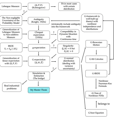
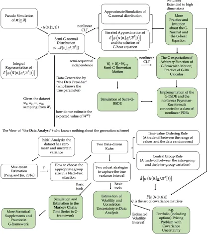
1.1 Overview of the Background and the Position of My Current Research . . . 1
1.2 My Current Research and Future Development . . . 9
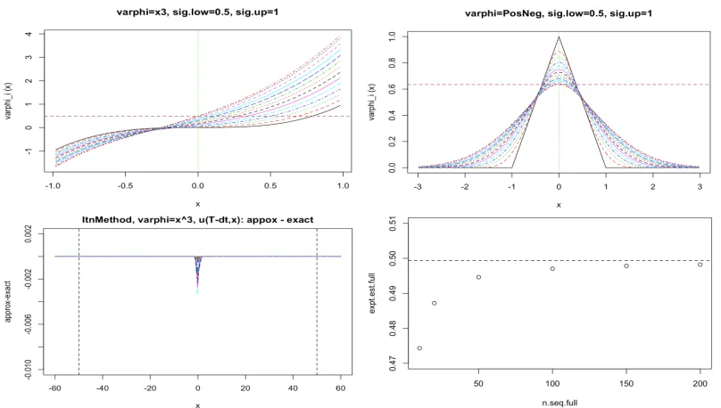
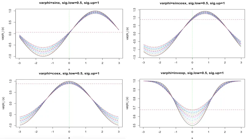
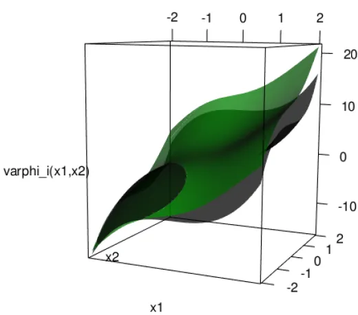
2.1 Numerical solution paths ofG-heat equation from our iterative method (Set I) . 35 2.2 Numerical solution paths ofG-heat equation from our iterative method (Set II) . 36 2.3 The numerical solution surface of the 2-dimensionalG-heat equation with initial functionϕ(x1,x2) = x31+ x32 . . . 37
3.1 The time-index plot of the first 1000 points of the dataset . . . 49
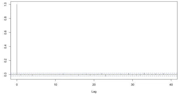
3.2 The autocorrelation function plot of the dataset to investigate possible linear autocorrelation . . . 49
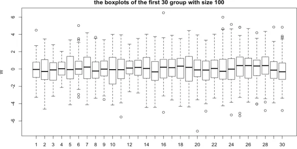
3.3 The boxplot of the first 30 groups with size 100 for the dataset . . . 50
3.4 The boxplot of the first 30 groups with size 100 for the square of the dataset . . 50
3.5 The sample variances against increasing sample sizen . . . 50
3.6 Black-box situation: the data provider vs the data analyst . . . 51
3.7 The change of max-mean estimations whenn=1,2, . . . ,√N. . . 53
3.8 Central group estimation . . . 55
3.9 Sampling distribution of the central group estimators . . . 56
3.10 Time-value ordering estimation . . . 57
3.11 Sampling distribution of the time-value ordering estimators . . . 58
4.1 Simulated sample of M[1,2] with large block length . . . 65
4.2 Simulated sample of M[1,2] with small block length . . . 65
4.3 A sample sequence from ˆN(0,[1,4]) . . . 67
4.4 Central group estimation of the variance uncertainty interval of ˆN(0,[1,4]) . . 67
4.5 A sample sequence from N(0,[1,4]) . . . 68
4.6 Central group estimation of the variance uncertainty interval of N(0,[1,4]) . . 69
A.1 Sampling distribution of the central group estimators with small true parameters 77 A.2 Sampling distribution of the time-value ordering estimators with small true parameters . . . 78
1.1 The two gambles (Urn I) . . . 2
1.2 The first pair of gambles (Urn II) . . . 3
1.3 The second pair of gambles (Urn II) . . . 3
1.4 Summary ofG-frame compared with Classical frame . . . 8
Introduction
1.1
Background of the
G
-framework
Figure 1.1: Overview of the Background and the Position of My Current Research
1.1.1
A simple story: What is
Uncertainty
?
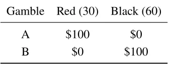
For general readers, let us start from a very simple example (which is taken from Ellsberg (1961)). Here we have an urn (called Urn I) containing 30 red balls and 60 black balls. One ball will be randomly drawn from the urn, then the colour of the ball will decide the money you get. Give you two gambles to consider (Table 1.1).
Table 1.1: The two gambles (Urn I)
Gamble Red (30) Black (60)
A $100 $0
B $0 $100
Gamble A or B, which one do you prefer? I bet it should not take you even a second to choose Gamble B or “a bet on black” (as long as you do not hate money). I also believe most readers (who prefer $100 to $0) will give me this obvious reason: Since the ball is more likely to be black, why not bet on black to get that $100 with higher chance?
In fact, this is one of the common senses in gambling strategies, which appeared even far before the notion calledprobability. The requirements of making better strategies in gambling
practice has actually motivated the early study of probability. To systematically describe stochas-tic phenomena in a more rigorous way, Kolmogorov (1956) constructed the axiomastochas-tic system of probability theory (which we call the classical probability framework) based on the additive Lebesgue measure. As we know, this classical framework gives a complete construction of the random variables and expectation. We can actually use the language of the classical probability framework (which should not be hard for any students with elementary probability knowledge) to explain and describe people’s preference in the scenario of Urn I (which is shown as follows). In the classical probability space (Ω,F,P), let X : Ω → {0,100} be a random variable
representing your income after the experiment. Since each ball in the urn has equal chance to be drawn, in Gamble A, the distribution ofX can be described by the following probability law
mappingPA:
X 100 0
PA 1/3 2/3
!
. (1.1)
Hence, the expected income in Gamble A can be expressed by the classical expectation of X
under the law PA, namely,EA[X]= 100×PA(X =100)+0×PA(X =0)= 100/3. Similarly,
for Gamble B, we have the probability lawPB:
X 0 100
PB 1/3 2/3
!
. (1.2)
Then the expected income from Gamble B isEB[X]= 200/3. In most people’s mind, in order
to maximize their “expected income”, they prefer Gamble B to A because of the underlying quantified relationEB[X]> EA[X]. This is also a simplified version of theexpected utility theory
(established by Von Neumann and Morgenstern (1945)) through defining a utility function
such thatU(100) >U(0)). In general, people choose one strategy if and only if it can maximize their expected utility. In the setting of Urn I, people prefer B to A if and only if B has larger expected utility or explicitly,EB[U(X)]> EA[U(X)] (if they are equal, people should not have
any preference over these two gambles), which is equivalent toPB(X = 100) > PA(X = 100).
Considering the probability regarding the colors the ball we draw might be and the rules in Table 1.2 (Gamble B is “a bet on black” and Gamble A is “a bet on red”), people prefer B to A if and only if P(draw a black ball) > P(draw a red ball) (they believe it is more likely to draw a black ball than a red one), which is consistent with the common gambling intuition.
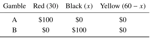
Let us do one step further and turn to another urn (called Urn II) containing 30 red balls and 60 balls that are black and yellow (in some fixed butunknown proportion). Suppose we have x
black balls and 60−xyellow balls wherexis some unknown integer in [0,60]. Again, one ball
is to be randomly drawn from the urn, the colour of which determines the money you get. You are provided with two gambles to reflect on, illustrated by Table 1.2.
Table 1.2: The first pair of gambles (Urn II)
Gamble Red (30) Black (x) Yellow (60−x)
A $100 $0 $0
B $0 $100 $0
Gamble A is “if the ball is red, you get $100, otherwise you get nothing” where we know there are 30 red balls. Gamble B is “if the ball is black, you get $100, otherwise nothing” where we only know there are [0,60] black ones. Do you prefer Gamble A or B? In other words, do you prefer “a bet on red” or “a bet on black”?
Now consider another pair of gambles C and D (Table 1.3).
Table 1.3: The second pair of gambles (Urn II)
Gamble Red (30) Black (x) Yellow (60−x)
C $100 $0 $100
D $0 $100 $100
Gamble C is a bet on “not black” and Gamble D is a bet on “not red”. Which of them do you prefer? (Take your time!)
According to the results from Ellsberg (1961), we have two common responses:
1. Response i(very frequent): Gamble A is preferred to B and Gamble D is preferred to C;
2. Response ii(less frequent): Gamble B is preferred to A and Gamble C is preferred to D.
Response i, people prefer Gamble A to B if and only if they believe drawing a red ball is
more likely than drawing a black one (“Reds are more than Blacks”). However, they also prefer Gamble D to C which is equivalent to their belief that it is more likely to draw a black ball than a red one (“Blacks are more than Reds”). This leads to a contradiction.
To better show the contradiction, if we apply the theory ofclassical expected utilitytheory,
again, we first need to set a utility functionU : 0,100→Rsuch thatU(100) >U(0)intuitively meaning people prefer $100 to $0. For instance, let
U(x)= I{x=100} B
1 x =100
0 x =0 .
We still useX to denote your income after the experiment, based on the unknownxand letting
y B x/90(∈[0,2/3])which is the proportion of black balls. The distribution of X andU(X), under different gambles, can be summarized by the following probability laws:
* . . . . . . . . . ,
X 0 100
U(X) 0 1
PA 2/3 1/3
PB 1−y y
PC y 1−y
PD 1/3 2/3
+ / / / / / / / / / -. (1.3)
Associated with the law (1.3) we also have, under probability P, EP[U(X)] = EP[I{X=100}] =
1× P(I{X=100} = 1) = P(X = 100). Then according to the theory of expected utility, people’s
preferences are characterized by maximizing the expected utility.Response ishowing Gamble
A is preferred to B indicates EA[U(X)] > EB[U(X)], which, by the probability law (1.3), can
be expressed asPA(X =100) > PB(X = 100)which is equivalent to 1/3 > y. We know ycan
be treated asthe unknown proportion of black ballsso “A is preferred to B” can be explained
by
the proportion of black balls < 1/3.
Meanwhile,Response i also says Gamble D is preferred to C then ED[U(X)] > EC[U(X)],
which meansPD(X = 100) > PC(X = 100)implying 2/3> 1−yor
the proportion of black balls > 1/3.
This leads to an obvious contradiction! (Noting that Urn II is not in some quantum world, although the number of black balls in Urn II is unknown, it should be some fixed one.) Readers can check Response ii also gives a logically similar contradiction. Both of them violate the
theory of classical expected utility.
Wait a moment. I know perhaps you were not really doing this kind of computation, since the proportion of black balls is unknown, how can we “pre-define” the threshold ofyto compare
the expected utility of two gambles? If not this, what kind of struggling was happening in your mind just now to make the strategy?
Actually, people (who giveResponse i and ii) usually tend to treat the proportion of black
and best cases). The unknown proportion of black balls is theuncertaintyhere since we do not
have information about this. In this spirit, the probability law (1.3) should be changed to a new version with “uncertainty”:
* . . . . . . ,
Gamble P(X =100)
A 1/3
B [0,2/3] C [1/3,1]
D 2/3
+ / / / / / / -. (1.4)
In Gamble A versus B, some people prefers Gamble A because they worry about the lower bound of the uncertainty interval given by B; (“what if there is no black balls, then I have no chance to get the money in B, at least Gamble A has 1/3 win rate.”) This kind of worry makes them they hate the uncertainty in B. This type of people have the so-calleduncertainty aversion, then they will be in favour of D in the comparison between Gamble C and D to avoid
the uncertainty in Gamble C (especially the lower bound).
Explicitly speaking, people with uncertainty aversion actually think about the “worst case” of all possible scenarios. For instance, in Gamble B, their “expected utility” in the worst case is actually theminimumof expected income in all possible settings ofy, motivating us to reflect
on a set of distributions or probability laws, namely, QB B {PB : PB(X =0) =1− y,PB(X =
100) = y,y ∈[0,2/3]}, rather than the single distribution ofXin Urn I governed by the law (1.1)
or (1.2). Then the “expected utility” can be written as ˆ
EB[U(X)] B min
PB∈QB
EPB[U(X)]= min
y∈[0,2/3]y =0. (1.5)
For Gamble A, since we only have one probability law for X (with no uncertainty), the set of
distributionsQA B {PA : PA(X = 0) = 2/3,PB(X = 100) = 1/3} degenerates to a singleton,
so the expected income is ˆ
EA[U(X)] B EPA[U(X)]=1/3. Therefore, we have
ˆ
EA[U(X)]> EˆB[U(X)], (1.6)
which describes the preference of people with uncertainty aversion in Gamble A versus B. Similarly, when people considering “the worst case” meet with Gamble C and D, sinceQC B
{PC :PC(X = 0) = y,PB(X =100) =1− y,y ∈[0,2/3]}, the expected income is
ˆ
EC[U(X)] B min
PC∈QC
EPC[U(X)]= min
y∈[0,2/3]1−y =1/3,
while the expected gain of Gamble D is ˆ
ED[U(X)] B EPD[U(X)]=2/3, so we have
ˆ
ED[U(X)]> EˆC[U(X)]. (1.7)
Meanwhile, there are another type of people (perhaps less frequent) preferring Gamble B to
seek the uncertaintyin it especially its upper bound; (“what if there is 60 black balls, then I have
2/3 chance, doubling the rate I get from A.”) This inclination will also drive them to choose C when comparing Gamble C and D. These type of people have the feature calleduncertainty seeking, whose expected utility can be expressed by the maximum of all possible cases since
they are looking for the “best income”, so we only need to change the minimum to maximum in Equation (1.5) to mathematically describe their preference.
Actually, the expectation ˆEin Equation (1.5) can be treated as theChoquet expectation(so
is the one replacing min with max), which is a nonlinear expectation able to be represented as the supremum (or equivalently, infimum, by adding a minus sign before the random variable) of a class of linear expectations under additive probability measures. Choquet (1954) generalizes the Lebesgue integral to non-additive measures so as to get the Choquet expectation.
1.1.2
Literature review: How do we deal with
Uncertainty
?
I will briefly review the historic development of the methodology to deal with uncertainty (also shown in Figure 1.1), in which the order and meaning of events partially refers to the survey by Peng (2017).
Knight (1921) gave the notion of Knightian Uncertainty (also known as Ambiguity in
finance) to distinguish it fromriskin his work Risk, Uncertainty, and Profit by saying:
“Uncertainty must be taken in a sense radically distinct from the familiar notion of Risk, from which it has never been properly separated.... The essential fact is that ’risk’ means in some cases a quantity susceptible of measurement, while at other times it is something distinctly not of this character.”
After the journey we have in Section 1.1.1, you may notice that the unknown proportion of black balls in Urn II exactly brings us the uncertaintyin the distribution of the income X,
forcing us to consider asetof distributions to characterize or cover this uncertainty. In fact, what
we played with Urn II is the famousEllsberg Paradoxwhich is a mind experiment proposed by
Ellsberg (1961), showing the violation of von Neumann-Morgenstern expected utility theory in the scenario with uncertainty and strongly motivating the construction of the new theory of expected utility under the Choquet expectation by Schmeidler (1989) later on.
However, the methods based on Choquet expectation cannot deal with the uncertainty in dynamic situations(especially with continuously changing time) because it is difficult to define
the conditional Choquet expectation (conditional on the filtration until time t), but the real
world we are facing has fundamental dynamic features. Fortunately, Chen and Epstein (2002) efficiently made progress in this problem in the setting of a sublinear expectation defined through the BSDE (Backward Stochastic Differential Equation) calledg-expectation (initially
developed by Peng (1997)), which nicely borrows the dynamic property of BSDEs to define its conditional expectation.
In principle,g-expectation can deal with any set of probability measures{Pθ}θ∈Θdominated
by a reference probabilityP. Nonetheless,g-expectation will fail when stepping into thesingular
scenario (that is, there exists an event Asuch thatP(A) =0 but Pθ(A) > 0), which is common in practice like the problem withvolatility uncertainty.
-expectation governed by BSDEs). It took researchers many years to realize that it is necessary to jump out of the Kolmogorov’s system(Ω,F,P), start from scratch and directly construct a new generalized probability framework to describe the uncertainty, which was established by Peng (2004, 2007a, 2008) and further developed by the academic group led by him, called the
G-expectation framework (Ω,H,Eˆ).
In the past two decades (since its establishment in 2000s), the G-expectation framework
has developed into a complete probabilistic structure with its own stochastic calculus and connection with a large family of nonlinear PDEs. It starts from theG-expectation (or sublinear
expectation) ˆE to redefine what are independence and identical distribution, from which it
induces the nonlinear version of “constants” (Maximal distribution with mean-uncertainty) and “normal distribution” (G-normal distribution with variance uncertainty). The independence in
this framework has thesequential orderwhich usually can not be reversed. Intuitively, this kind
of design partially comes from the spirit of backward analysis similar to the analysis in BSDEs. From the starting axioms of(Ω,H,Eˆ), we are able to completely and systematically construct all the basic and important results in probability, stochastic analysis and statistical theory, which actually give a brand-new understanding of those stochastic concepts under the uncertainty setting and also generalize the classical results in a non-trivial way with much weaker and more general conditions. Specially speaking, theG-framework has its own probabilistic inequalities,
Central Limit Theorem (CLT) (Peng (2007b), Hu and Zhou (2015)) with convergence rate by Song (2017), Law of Large Numbers (LLN) (Chen et al. (2013)) and also G-Itô-stochastic
calculus based on the construction of G-Brownian motion (Denis et al. (2011)), in which
there are diffusion processes driven by G-Brownian motion including the BSDEs, the so
called G-BSDEs. More complete collection of results can be found in Peng (2007a, 2008).
Furthermore, similar to the counterparts in classical framework, Hu et al. (2014) shows that the
G-BSDEs are connected by the Feynman-Kac formula inG-framework with a large class of fully
nonlinear PDEs (able to be applied to control problems with uncertainty, especially in financial background). If we can numerically solve theG-BSDEs, it is very promising that we will be
able to stochastically solve the high-dimensional fully nonlinear PDEs (whose nonlinearity and curse of dimensionality make most classical numerical PDE methods fail).
However, problems are arising from both the academy and industry:
1. If the G-framework intends to deal with the problems with uncertainty, given a real
problem with dataset, how can we do the estimationof those parameters to fit into the
setting ofG-framework?
2. If the G-Brownian motion and the G-BSDE are able to cover or capture the volatility
uncertainty (especially solving those nonlinear PDEs), is it possible to simulate the G
-Brownian motion (or theG-normal distribution) as well as theG-BSDE, and how do we
compute the correspondingG-expectation of thoseG-itô integral?
Before answer the questions above, we need to consider a crucial one:
How do we statistically and numerically deal with the distributions in theG-framework?
Typically, how can we better understand and handle theG-normal distribution? Actually, another
key problem hidden here is thesequential independenceattached with the distributions. We may
industrial problems with uncertainty and the implementation of the new stochastic nonlinear PDE methods based on the diffusion processes in the G-framework. This thesis is exactly
trying to explore the computational and statistical methodology in theG-framework, especially
starting from theG-normal distribution (a typical one with variance uncertainty).
The computation of the G-expectation based on a given parameter setting has been
de-veloped for several years like the numerical schemes by Dolinsky (2012) to approximate the
G-expectation. In fact, due to the nonlinearity of the expectation and the uncertainty intrinsically
included in the distributions, the statistical theory in theG-framework is not easy or trivial to
develop. So far there are already some attempts like the Max-mean estimation by Jin and Peng (2016) aimed at estimating the parameters or the sublinear expectations from dataset but it still requires the context of real data to offer more information about how to do the grouping and decide the test function. (In this thesis, sometimes we stress “real” data to distinguish from the artificial data generated by ourselves.)
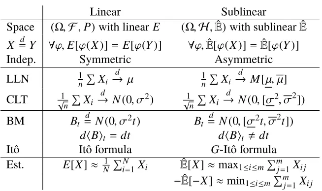
To summarize, Table 1.4 shows the existing objects and results in the G-expectation (or
sublinear expectation) framework compared with the counterparts in classical probability
framework (withlinearexpectation), where the concepts inG-frame will be further explained
in Section 2.1.
Table 1.4: Summary ofG-frame compared with Classical frame
Linear Sublinear
Space (Ω,F,P) with linearE (Ω,H,Eˆ)with sublinear ˆE
X =d Y ∀ϕ,E[ϕ(X)]= E[ϕ(Y)] ∀ϕ,Eˆ[ϕ(X)]=Eˆ[ϕ(Y)]
Indep. Symmetric Asymmetric
LLN 1n
P
Xi d
→ µ 1nP
Xi d
→ M[µ, µ]
CLT √1
n
P
Xi d
→ N(0, σ2) √1
n
P
Xi d
→ N(0,[σ2, σ2])
BM Bt
d
= N(0, σ2t) Bt d
= N(0,[σ2t, σ2t])
dhBit = dt dhBit , dt
Itô Itô formula G-Itô formula
Est. E[X]≈ N1 PN
i=1Xi Eˆ[X]≈max1≤i≤m
Pm
j=1Xi j
−Eˆ[−X]≈min1≤i≤mPmj=1Xi j
Let us start our exploration and adventure beginning with the G-normal distribution N(0,[σ2, σ2]), one of the basic objects in theG-framework, based on some existing theoretical
work by the pioneers, to design and construct a new basic substructure, the semi-G-normal
distribution, in order to provide statistical tools for the whole framework and also the larger community to better understand and study the variance uncertainty. Hope you will see some interesting, inspiring and delicate designs (such as the semi-G-normal distribution with its nice
1.2
Overview of my research
The main content of this thesis, aimed at exploring the computation, simulation and esti-mation ofG-normal distribution, consists of four chapters:
• Chapter 2: the distributions and independence in theG-framework;
• Chapter 3: the estimation of variance uncertainty;
• Chapter 4: the pseudo simulation of variance uncertainty; • Chapter 5: concluding remarks and future development.
Although theG-framework has strong potential to theoretically deal with ambiguity, because
of the sub-additivity ofG-expectation ˆE[·], it is hard to develop the statistical or computational
version of G-framework, which is the bridge to real data analyses and industrial problems.
This is especially true for theG-normal distribution X ∼ N(0,[σ2, σ2]), as itsG-expectation
ˆ
E[ϕ(X)] does not have an explicit expression if ϕ is neither convex nor concave. In order to
compute the ˆE[X2n+1], previously we needed to use special PDE and ODE techniques to solve
theG-heat equation (Hu (2012)).
Chapter 2 mainly investigates the distributions and independence in theG-framework and
establishes a substructure (Section 2.3) based on a new concept called the semi-G-normal distributionlike a transition from classical normal toG-normal distribution to fill in the thinking
gap between these two objects to get better intuition and do the computation and simulation of
G-normal distribution. It actually gives a probabilistic method (based on theG-framework) to
compute theG-expectation ofG-normal distribution. This is a great extension allowing us to deal
with theG-expectation of a larger class of functions ofG-normal distribution. Interestingly, this
substructure gives an efficient iterative scheme to stochastically solve, by Monte-Carlo method, theG-heat equation (which is fully nonlinear PDE, also known as theBlack-Scholes-Barenblatt equation with volatility uncertainty). Section 2.3 has also been written as a preprint paper (Li
and Kulperger (2018), which is mainly done by myself under the supervision of Prof. Kulperger) we intend to publish in the near future. We also explore the independence (Section 2.4) regarding
G-normal and semi-G-normal distribution, showing that one annoying property ofG-normal
distribution is that it not easy to constructmultivariateG-normal distribution fromunivariate
objects. Can we find a path to construct the multivariateG-normal distribution from univariate
objects? We will give a positive answer by showing how to start from the univariate semi-G
-normal objects, with its special design of independence, to approach the multivariateG-normal
distribution.
Then we come to the side of dataset including estimation (Chapter 3) and simulation (Chapter 4) which require and apply both the theory and intuition we have learned in Chapter 2. One important question regarding the real data analysis with variance uncertainty is, if treated asG-normal distribution, how to estimate the variance interval. Although the established
Max-mean method by Jin and Peng (2016) gives a theory of this kind of estimation, it still relies on the information from the practical background to decide the group size and test function.
Chapter 3 provides two heuristic data-driven rules (Section 3.2) for Max-mean estimation to appropriately select the group size so as to robustly capture the true variance interval, which turns out to numerically work well. We will further work on more practice of this improved Max-mean estimation and more theory to support it. Meanwhile, we also try to put the estimation method into practice so as to get more designing ideas from the application background.
Chapter 4 designs a simulation procedure centering around the semi-G-normal distribution,
of theG-normal distribution. The simulation is essentially important for the numerical testing
the estimation methods in Chapter 3.
Finally, Chapter 5 summarizes the whole thesis and discuss about the future development especially about the future industrial practice of theG-framework.
The Distributions and Independence in
the
G
-framework
2.1
Preliminaries
TheG-expectation or sublinear expectation framework (also called theG-framework), motivated
by the problems with ambiguity or uncertainty, is a generalization of the linear probability
framework. Similar to the Choquet expectation, the sublinear expectation can be represented as the supreme of a class of linear expectations. Intuitively, the linear expectation mainly considers the “average”, while the sublinear expectation focuses on the “bound” to create a interval to cover the uncertainty which is hard to be described by a certain distribution. Please turn to Peng (2004, 2007a, 2008, 2010) for more details.
Definition 2.1.1. Asublinear expectaion space is defined as a triple (Ω,H,Eˆ). Ω is a given
set (also known as a sample space).H is a linear space of real valued functions defined onΩ
satisfying c ∈ H for each constant c and |X| ∈ H if X ∈ H, which can be regarded as the
space of random variables. ˆE is a sublinear expectation which is a functional ˆE : H → Rd
satisfying:
1. Monotonicity: ˆE[X] ≥ Eˆ[Y] if X ≥Y;
2. Constant preserving: ˆE[c]=cforc ∈Rd;
3. Sub-additivity: For eachX,Y ∈ H, ˆE[X+Y] ≤Eˆ[X]+Eˆ[Y];
4. Positive homogeneity: ˆE[λX]= λEˆ[X] forλ ≥ 0.
If only monotonicity and constant preserving are satisfied, ˆEis called a nonlinear expectation
and(Ω,H,Eˆ) is called a nonlinear expectation space.
In this thesis, since we will not deal with nonlinear expectation (without sub-additivity and positive homogeneity), we will not strictly distinguish between “sublinear” and “nonlinear.” Therefore, in some casual context of the description of theG-framework, we may use “nonlinear”
and“sublinear” interchangably, as they are both distinguished from the word “linear”, which is the difference we mostly care about.
In fact, similar to Choquet expectation (for readers familiar with its setting), the sublinear expectation defined in Definition 2.1.1 can also be expressed as the supreme of a class of linear
expectations corresponding to a family of probability measures (Theorem 2.1.2). Choquet expectation is a special case of the sublinear expectation.
Theorem 2.1.2(Representation of sublinear expectation). LetEˆ denote a sublinear expectation
onH. Then there exists a family of probability measures Q which correspondingly induces a collection of linear expectation{EP, P ∈ Q}onH such that for each X ∈ H,
ˆ
E[X]= sup
P∈Q
EP[X].
Remark2.1.2.1. Meanwhile, for each X ∈ H, there existsθX ∈ Qsatisfying ˆE[X]= EθX[X]. In the following context, we often use capital letters like X B (X1,X2, . . . ,Xd),d ∈N+ to
denote the random variables (or vectors) inH. Meanwhile, ifX ∈ H, we also haveϕ(X) ∈ H
for everyϕinCl.Lip(Rd) which is the linear space of functions satisfying the locally Lipchistz
property:
|ϕ(x)−ϕ(y)| ≤ Cϕ|1+|x|k+ |y|k||x− y|,
for x,y ∈ Rd, somek ∈NandCϕ > 0 depending onϕ. If not specified, we will always stay in
thesublinear expectation space(Ω,H,Eˆ)and the function spaceCl.Lip(Rd)(orCl.Lipin short,
which can be replaced by other spaces). Our computation in this space is usually different from the linear expectation E mainly because of the sub-additivity and positive homogeneity of ˆE.
Here are some useful tools to understand and deal with ˆE.
In general, for any X ∈ H, we must have−Eˆ[−X] ≤ Eˆ[X] because 0 = Eˆ[X +(−X)] ≤
ˆ
E[X]+ Eˆ[−X]. Whether it is a strict inequality tells us whether X has “uncertainty” or not,
which is better illustrated by Definition 2.1.3.
Definition 2.1.3 (Moments-uncertainty). For each X ∈ H, we say X has the k-th moment-uncertaintyif−Eˆ[−Xk] < Eˆ[Xk] < ∞for k = 1,2, . . . ,n. X hasthek-th moment-certaintyif
−Eˆ[−Xk]= Eˆ[Xk]< ∞. Specifically, we have
1. X has mean-uncertainty (or mean-certainty, respectively) if it has the 1-st
moment-uncertainty (or 1-st moment-certainty, respectively);
2. When X satisfies 0 = −Eˆ[−X] = Eˆ[X], X has the variance-uncertainty (or
variance-certainty, respectively) if it has the 2-nd moment-uncertainty (or 2-nd moment-variance-certainty, respectively).
Proposition 2.1.4. If X has the mean-uncertainty: µ < µwith µ B −Eˆ[−X]and µ B Eˆ[X],
for λ∈R, we will have
ˆ
E[λX]=
λEˆ[X] λ ≥ 0
−λEˆ[−X] λ < 0 = λ
+µ−λ−µ,
whereλ+ Bmax{λ,0}andλ− B max{−λ,0}.
Proposition 2.1.5. If X has the mean-certainty: µ= µC µnamely−Eˆ[−X] = Eˆ[X] = µ, for λ∈R, we will have
ˆ
E[λX]= λEˆ[X](= λ µ),
and furthermore,
ˆ
Proof. The first one is directly from the mean-certain-1. For the second one, firstly we have
ˆ
E[Y +λX]≤ Eˆ[Y]+Eˆ[λX]=Eˆ[Y]+λEˆ[X].
Secondly since ˆE[Y]=Eˆ[Y −X+X]≤ Eˆ[Y −X]+Eˆ[X] implies ˆE[Y−X]≥ Eˆ[Y]−Eˆ[X], we
have
ˆ
E[Y +λX]=Eˆ[Y −λ(−X)]≥ Eˆ[Y]−Eˆ[λ(−X)]=Eˆ[Y]+λEˆ[X].
Combining the two inequalities, we get ˆE[Y +λX]=Eˆ[Y]+λEˆ[X].
In general, without any requirements like the mean-certainty of the random variables, we have the following probability inequalities (Proposition 2.1.6 and Proposition 2.1.7).
Proposition 2.1.6(Hölder inequality). For p,q> 0, 1p + 1q =1, we have
ˆ
E[|XY|] ≤ (Eˆ[|X|p])1/p(Eˆ[|Y|q])1/q.
Proposition 2.1.7(Minkowski inequality). For p≥ 1, we have
(Eˆ[|X +Y|p])1/p ≤ (Eˆ[|X|p])1/p+ (Eˆ[|Y|p])1/p. We will use ˆEto redefine distributions and independence.
Definition 2.1.8(Distributions). We give the notions of distribution, identical distribution and
convergence in distribution as follow.
1. FX is called the distribution of X, which is a functional: FX[ϕ] B Eˆ[ϕ(X)] : ϕ ∈ Cl.Lip(Rd) →R.
2. X andY areidentically distributed, denoted byX =d Y, if for anyϕ ∈Cl.Lip,
ˆ
E[ϕ(X)]= Eˆ[ϕ(Y)],
namely,FX[ϕ]=FY[ϕ].
3. A sequence {Xn}∞n converges in distribution to X, denoted as Xn
d
→ X, if for any ϕ ∈Cl.Lip,
lim
n→∞Eˆ[ϕ(Xn)]= Eˆ[ϕ(X)].
Definition 2.1.9 (Independence). Y is independent from X, denoted by X d Y, if for any ϕ∈Cl.Lip,
ˆ
E[ϕ(X,Y)]=Eˆ[ ˆE[ϕ(x,Y)]x=X].
Remark 2.1.9.1. For readers’ convenience, the notation ˆE[ ˆE[ϕ(x,Y)]x=X] means two steps of
computation:
1. for any fixedx, compute ˆE[ϕ(x,Y)] which becomes a function of xdenoted asH(x);
Comment 2.1.9.1. Intuitively, X d Y means that any realization of X will have no effect
onY’s uncertainty set of distributions. X d Y does not meanY d X. In other words, this
independence has its order. In the scenario of linear expectation, the notion of independence
in Definition 2.1.9 becomes the classical one. The sequential independence is one of the most important notions in the G-framework, about which, more exploration can be found in
Section 2.4.
Definition 2.1.10 (i.i.d.). {Xi}i∞=1 is i.i.d. if Xi+1 =d Xi and (X1,X2, . . . ,Xi) d Xi+1 for each
i ∈N+.
Let ¯X be an independent copy ofX, which means ¯X =d X and X d X¯.
Definition 2.1.11(Maximal distribution). X followsMaximal Distributionif, for any
indepen-dent copy ¯X, we have
aX +bX¯ =d (a+b)X ∀a,b≥ 0,
which is equivalent to
X+ X¯ =d 2X.
This is the sublinear version of a constant. A more specific definition with representation is given by Definition 2.1.12.
Definition 2.1.12 (Maximal distribution with representation). X follows the maximal
distri-bution M(Γ) if there exists a bounded, closed and convex set Γ ⊂ Rd such that for any
ϕ∈Cl.Lip(Rd),
FX[ϕ]=Eˆ[ϕ(X)]=max
v∈Γ Eδv[ϕ(X)]= maxv∈Γ ϕ(v),
whereδv is the Dirac measure with respect tov ∈ Rd. For d = 1, we have X ∼ M[µ, µ] with
mean-uncertainty: µB −Eˆ[−X] and µB Eˆ[X].
Definition 2.1.13(G-normal distribution). X followsG-normal Distribution if, for any
inde-pendent copy ¯X, we have
aX +bX¯ =d pa2+b2X, ∀a,b ≥0,
which is equivalent to
X +X¯ =d
√
2X.
For d = 1, we have X ∼ N(0,[σ2, σ2]) (0 ≤ σ ≤ σ) with variance-uncertainty: σ2 B
−Eˆ[−X2] andσ2 BEˆ[X2].
The Proposition 2.1.14 is a good practice for general readers to work on the new operator ˆE.
Proposition 2.1.14 (The scaling property ofG-normal distribution). Let X ∼ N(0,[σ2, σ2]), then for any given constant c ∈ R, we have cX ∼ N(0,[c2σ2,c2σ2]) which, by using the simplified notationc[σ, σ] B [ca,cb], can be written as
Proof. Firstly, we need to showY B cX is alsoG-normal distributed. For any independence
copy ¯Y, it can be equivalently written ascX¯ (readers can prove the two deductive directions),
where ¯X is also an independent copy of X. Then we have
Y +Y¯ = cX +cX¯ = c(X +X¯)=d c
√
2X =
√
2Y.
Secondly, compute the two bounds of variance interval ofY:
ˆ
E[Y2]=Eˆ[(cX)2]= Eˆ[c2X2]=c2Eˆ[X2]=c2σ2,
and
−Eˆ[−Y2]=−Eˆ[−(cX)2]=−Eˆ[c2(−X2)]=−c2Eˆ[−X2]=c2σ2.
Therefore,Y = cX ∼ N(0,[c2σ2,c2σ2]).
LetSddenote the set of all real-valued d×d symmetric matrices andS+d(⊂ Sd)represent
the set of non-negative definite symmetric matrices.
Theorem 2.1.15(G-normal distribution characterized by the G-heat Equation). X follows the
d-dimensionalG-normal distribution, iffu(t,x) B Eˆ[ϕ(x+
√
1−t X)]is the (unique viscosity) solution totheG-heat Equationdefined on[0,∞)×Rd:
ut+G(D2xu) =0, u|t=1= ϕ,
where G(A) B 12Eˆ[hAX,Xi] : Sd → R, which is a sublinear function characterizing the
distribution of X. Ford = 1, we haveG(a) = 12(σ2a+ −σ2a−)and whenσ2 > 0, this is also calledthe Black-Scholes-Barenblatt equationwith volatility uncertainty.
Remark2.1.15.1. We can use the functionG(A) B 21Eˆ[hAX,Xi] to characterize the definition
ofG-normal distribution. In fact,G(A)can be further expressed as
G(A) = 1 2Vsup∈V
tr[AV],
whereV = {BBT :B∈Sd}is a collection of non-negative definite symmetric matrices which
can be treated as the uncertainty set of the covariance matrices.
Comment2.1.15.1. In Theorem 2.1.15, we use the notion ofviscositysolution as a replacement
of the classical one when lacking smoothness because of the nonlinearity of theG-heat equation.
The definitions and more details of viscosity solution can be found in Crandall et al. (1992). From Peng (2010), whenGis non-degenerate, the viscosity solution becomes a classicalC1,2
solution. Since this thesis has not touched or stressed a lot on the differences between the viscosity and classical solutions yet, readers who are not familiar with viscosity solutions can simply treat this notion as the classical ones in the following context.
Remark2.1.15.2 (A direct origin and application of theG-heat equation, Avellaneda and Paras
(1996)). In fact, the form of theG-heat equation is not some brand-new design but was actually
Volatility Model (UVM) is well-worth mentioning here. Consider a model valuing a contingent claim based on an underlying asset with volatility uncertainty. Suppose the spot price of the underlying asset follows a stochastic differential equation:
P : dSt St =
µtdt+σtdZt,
with µt = rt−dt (wherert is the spot domestic riskless rate and dt is the dividend rate). The
volatility process is assumed to fluctuate within a band
σ ≤ σt ≤ σ,0 ≤t ≤T.
Consider an agent that must deliver a stream of cash-flowsF1(Sti),i = 1,2, . . . ,N whereFj(·) are payoffs due at settlement datest1< t2< . . . <tN. The worst case scenario present value is
V(St,t)= sup P∈Q EP N X
j=1
exp(−r(tj −t))Fj(Stj)
.
Actually,V(S,t)satisfies the nonlinear programming equation (similar to theG-heat equation):
Vt+ 1
2σ2(VSS)·VSS+ µSVS−rV =0,
where
σ2(VSS) =
σ2 ifVSS ≥ 0
σ2 ifV
SS <0
.
Another equivalent form is easier for us to treat it as a PDE in control theory (HJB equation):
Vt+ sup
σ2∈[σ2,σ2]
(1
2σ2VSS)+ µSVS−rV =0.
Definition 2.1.16(G-normal distribution with characterization). Let X be any d-dimensional G-normal distributed random vector. To be specific, we say X ∼ N(0,V) with the set of covariance matricesV if its distribution is characterized by theG-heat equation with
G(A) B 1
2Eˆ[hAX,Xi]= 1 2Vsup∈V
tr[AV].
In other words,V is the set corresponding to theGfunction characterizing the distribution of X. In order to show thecovariance-uncertaintyofN(0,V), we can expand the details ofV as
V B
V= ρi jσiσj
d×d : σ
2
i ∈[σ2i, σ2i],
ρi j = ρji =
1 i = j
∈[ρ
i j, ρi j] i , j
, such thatV∈S+d
.
Whend = 1, we sayX ∼ N(0,[σ2, σ2])with the variance interval [σ2, σ2] if its distribution is characterized by theG-heat equation with
Based on the G-version of “constant” and “normal” distribution, we have the respective
Law of Large Numbers (LLN) and Central Limit Theorem (CLT) in theG-framework.
Theorem 2.1.17 (Law of Large Numbers, Peng (2010)). Consider a sequence of i.i.d. {Zi}i∞=1 withmean-uncertaintycharacterized by a (unique) bounded, closed and convex setΓ ⊂ Rd in the sense that
max
v∈Γhp,vi=
ˆ
E[hp,Z1i],p∈Rd.
Then for anyϕ ∈Cl.Lip,
lim
n→∞Eˆ[ϕ(
1
n
n
X
i=1
Zi)]=Eˆ[ϕ(Z)],
where Z is a maximal distributed random variable characterized by the setΓ:
ˆ
E[ϕ(Z)]=max v∈Γ ϕ(v).
For d = 1, Γ becomes a closed interval [µ, µ] with µ B −Eˆ[−Z1]and µ B Eˆ[Z1]. Then we
have 1nPn
i=1Zi)converges in distribution toZ ∼ M[µ, µ].
Theorem 2.1.18(Central Limit Theorem, Peng (2010)). Consider a sequence of i.i.d.{Xi}i∞=1 with mean-certaintyEˆ[X1]= −Eˆ[−X1]= 0. LetX be aG-normal distributed random variable
characterized by the functionG(A) B 12Eˆ[hAX1,X1i]. Then for anyϕ ∈Cl.Lip,
lim
n→∞Eˆ[ϕ(
1
√
n
n
X
i=1
Xi)]= Eˆ[ϕ(X)].
For d = 1, let σ2 B −Eˆ[−X12] and σ2 B Eˆ[X12]. Then we have √1
n
Pn
i=1Xi converges in distribution toX ∼ N(0,[σ2, σ2]).
We will call Theorem 2.1.18 the nonlinear CLT. We also have the convergence rate of nonlinear CLT.
Theorem 2.1.19 (The convergence rate of nonlinear CLT by Song (2017)). Under the setting of Theorem 2.1.18 when d = 1, for bounded and Lipschitz continuousϕ(i.e. for any x,y ∈ R,
|ϕ(x)| ≤ M and|ϕ(x)−ϕ(y)| ≤ Cϕ|x−y|), there existα∈ (0,1)depending onσandσ, and
Cα,G > 0depending onα,σandσsuch that
sup
Cϕ≤1
ˆ
E[ϕ(√1 n
n
X
i=1
Xi)]−Eˆ[ϕ(X)]
≤ Cα,G
ˆ
E[|X1|2+α]
nα2 =O(
1
nα2 ).
2.2
Motivation: How can we better understand the
G
-normal
distribution?
For the academic community concerning the G-framework, there is a long existing thinking
For instance, according to the comparison theorem of parabolic PDEs given by Crandall et al. (1992), it is not hard to show
ˆ
E[ϕ(N(0,[σ2, σ2]))] ≥ sup
σ∈[σ,σ]E[ϕ N(0, σ 2))],
which indicates that the uncertainty set ofG-normal distribution is much larger that a class of
lin-ear normal distributions withσ ∈[σ, σ] (so what else is in theG-normal set of distributions?).
Especially, Hu (2012) shows the strict inequality that whenϕ(x)= x3,
ˆ
E[ N(0,[σ2, σ2])3] >0.
According to Proposition 2.1.14, letX =d N(0,[σ2, σ2])then we have−X =d N(0,[σ2, σ2]), namely,
X =d −X, (2.1)
which indicates that theG-normal distribution should have some “symmetry”. However, exactly
due to this identity in distribution shown in Equation (2.1), from Definition 2.1.8, we have ˆ
E[−X3]=Eˆ[(−X)3)]=Eˆ[X3](> 0),
which directly implies, (letting E and N(0, σ2) respectively denote the classical expectation and normal distribution,)
ˆ
E[ N(0,[σ2, σ2])3]> 0= E[ N(0, σ2)3]> −Eˆ[− N(0,[σ2, σ2])3].
telling us that the “skewness” ofG-normal distribution becomes uncertain so its “symmetry”
is uncertain, which somehow looks like a “contradiction” with Equation (2.1) and is quite counter-intuitive for a “normal” distribution.
Is it possible to understand the G-normal distribution from our familiar classical normal
distribution? In other words, is it possible to use the linear expectation of linear normal dis-tribution (or the heat equation) to approach the sublinear expectation ofG-normal distribution
(or the G-heat equation)? This section gives positive answers to both of these questions by
providing a ladder from the ground of N(0, σ2) to approach the peak of N(0,[σ2, σ2]): the
Semi-G-normaldistribution ˆN(0,[σ2, σ2]), which is a classical normal distribution scaled by a sublinear “constant” (the maximal distribution).
2.3
The semi-
G
-normal distribution and
G
-normal
distribu-tion
2.3.1
The
1
-dimensional situation
Definition 2.3.1(The Semi-G-normal Distribution). Wfollows theSemi-G-normal distribution,
denoted as,W ∼ Nˆ(0,[σ2, σ2]), if there existY ∼ N(0,[1,1]) and Z ∼ M[σ, σ], σ ≥ σ ≥ 0
with independent relation Z dY, such that
W = Z ·Y,
where “·” is the number multiplication (which can be omitted) and the direction of independence
Remark2.3.1.1. Y ∼ N(0,[1,1]) can be regarded as the classical standard normal distribution
N(0,1)since the correspondingG-heat equation will reduce to the classical heat equation when σ andσcoincide.
Remark 2.3.1.2 (the mean and variance ofW). It is not hard to show that it has a certain zero
mean:
ˆ
E[W]=Eˆ[ZY]=Eˆ[ ˆE[zY]z=Z]=Eˆ[E[zY]z=Z]=0,
and−Eˆ[−W]=0. For the variance, we have
ˆ
E[W2]=Eˆ[Z2Y2]= Eˆ[ ˆE[z2Y2]z=Z]=Eˆ[E[z2Y2]z=Z]= Eˆ[(z2·1)z=Z]= max z∈[σ,σ]z
2 =σ2,
and similarly,
−Eˆ[−W2]=Eˆ[−Z2Y2]=−Eˆ[E[−z2Y2]z=Z]= − max z∈[σ,σ](
−z2) = min
z∈[σ,σ]z
2= σ2.
Theorem 2.3.2 (The Integral Representation of the Semi-G-normal Distribution). Let W ∼
ˆ
N(0,[σ2, σ2])then for anyϕ ∈Cl.Lip(R), we have
ˆ
E[ϕ(W)]= max
z∈[σ,σ]E[ϕ(N(0,z
2))]= max
z∈[σ,σ]
Z ∞
−∞
1
√
2πe
−y2/2ϕ(
zy)dy.
Proof. This is quite straightforward because:
ˆ
E[ϕ(W)]=Eˆ[ϕ(Y Z)]=Eˆ[ ˆE[ϕ(Y z)]z=Z] CEˆ[G(Z)],
whereG(z) B Eˆ[ϕ(Y z)]= E[ϕ(N(0,z2))] can be proved to be inCl.Lipbased onϕ ∈ Cl.Lip .
Specifically, we have
|G(x)−G(y)| = |E[ϕ(x· Z)−ϕ(y·Z)]|
≤ E[Cϕ(1+|x Z|k+|yZ|k)|Z| · |x− y|] =Cϕ·E[|Z|+|Z|k+1|x|k +|Z|k+1|y|k]|x− y| ≤ CG(1+|x|k+|y|k)|x−y|,
whereCG =Cϕmax{E[|Z|],E[|Z|k+1]}. Therefore,
ˆ
E[ϕ(W)]= Eˆ[G(Z)]= max
z∈[σ,σ]G(z) = max
z∈[σ,σ]E[ϕ(N(0,z
2))]
= max
z∈[σ,σ]
Z ∞
−∞
1
√
2πe
−y2/2ϕ(zy)dy.
Remark2.3.2.1 (Why is it called a “semi” one?). The comparison theorem of parabolic PDEs
(in Crandall et al. (1992)) tells us that ˆ
E[ϕ(N(0,[σ2, σ2]))]≥ max
v∈[σ,σ]E[ϕ(N(0,v
2))]= ˆ
E[ϕ(Nˆ(0,[σ2, σ2]))],
whose inequality is mostly strict (like ϕ(x) = x3) and becomes equal when ϕ is convex or
concave. From the representation theorem of ˆE: ˆE[ϕ(X)]= supP∈QEP[ϕ(X)], we have the
in-tuition thatQSemi-G-normal ⊂ QG-normalwhereQSemi-G-normalconsists of measures corresponding
Remark 2.3.2.2. Intuitively, the G-normal distribution is more “uncertain” than the semi-G
-normal distribution. Explicitly speaking, we already have the following representation for the
G-normal distributedX ∼ N(0,[σ2, σ2])(Denis et al. (2011) and Li (2015)) which is consistent with the spirit of the uncertain volatility model mentioned in Remark 2.1.15.2:
ˆ
E[ϕ(X)]= sup θ∈AΘ
EP[ϕ(
Z 1
0 θsdBs)],
whereΘ=[σ, σ], AΘ B {θ :θt ∈Θ,fort ∈[0,1]}, the set of all processes valuing in [σ, σ] in
the time range [0,1] andBis the classical Brownian motion in(Ω,F,P). Meanwhile, from the integral representation (Theorem 2.3.2), we can show that forW ∈ Nˆ(0,[σ2, σ2]),
ˆ
E[ϕ(W)]= sup θ∈AΘ
EP[ϕ(
Z 1 0
¯
θdBs)],
where ¯θ = R 1
0 θsds(∈ [σ, σ]), the average of the process θ over the time interval [0,1].
To summarize, the G-normal distribution has the uncertainty set consisting of all processes
valuing in Θ, while the semi-G-normal distribution only has the set made up of all constant processesvaluing inΘ.
Corollary 2.3.2.1(the connection with theG-normal distribution). Whenϕis convex or concave andϕ ∈C2(R), for X ∼ N(0,[σ2, σ2])andW ∼ Nˆ(0,[σ2, σ2]), we have
ˆ
E[ϕ(X)]=Eˆ[ϕ(W)].
Proof. The proof consists of two parts: first show the sublinear expectation ofG-normal
distri-bution and then gives the expectation of semi-G-normal distribution to prove their coincidence.
The sublinear expectation of G-normal distribution: Under convexity (or concavity), the
integral representation ofG-normal distribution directly comes from the solution of the classical
heat equation because u(t,x) will be convex (or concave, respectively) to x thenux x ≥ 0 (or
≤0, respectively) (more details can be found in Peng (2010)), giving us
ˆ
E[ϕ(X)]=
E[ϕ(N(0, σ2))] ϕis convex
E[ϕ(N(0, σ2))] ϕis concave,
for which we give a scratch proof here to general readers with interests. According to Theo-rem 2.1.15, the sublinear expectation ofG-normal distribution can be treated as the solution
of a nonlinear PDE called the G-heat equation (or sometimes in one dimension called the Black-Scholes-Barenblatt equation with volatility uncertainty). Explicitly speaking, after a time
transformation, for X ∼ N(0,[σ2, σ2]),u(t,x) B Eˆ[ϕ(x+
√
t X)] becomes the (unique viscos-ity) solution of theG-heat equation defined on [0,∞)×Rd:
ut− 1
2(σ2u+x x −σ2u
−
x x)= 0,u|t=0 =ϕ,
or equivalently,
ut− sup
σ∈[σ,σ]
{1
When ϕ is convex, (that is, for any x,y ∈ R and a ∈ [0,1], ϕ(ax + (1− a)y) ≤ aϕ(x) + (1− a)ϕ(y)), we can check thatu(t,x) is also convex with respect to x: for any x,y ∈ Rand
a ∈[0,1],
u(t,ax+(1−a)y) =Eˆ[ϕ(ax+ (1−a)y+
√
t X] =Eˆ[[ϕ(ax+ (1−a)y+
√
tc]c=X]
=Eˆ[[ϕ(a(x+
√
tc)+(1−a)(y+√tc)]c=X]
≤ Eˆ[[aϕ(x+√tc)+(1−a)ϕ(y+√tc)]c=X]
=Eˆ[aϕ(x+
√
t X)+(1−a)ϕ(y+√t X)]
≤ aEˆ[ϕ(x+
√
t X)]+(1−a)Eˆ[ϕ(y+
√
t X)]
=au(t,x)+(1−a)u(t,y).
As mentioned in Comment 2.1.15.1, under some non-degenerate conditions, the viscosity solutionu(t,x)isC1,2. Then we haveux x ≥ 0 so thatu−x x = 0 and Equation (2.2) degenerates to
a classical one:
ut− 1
2σ2ux x =0,u|t=0 = ϕ,
which is a Cauchy problem of theclassical heat equation with a nice explicit unique solution
in terms of the Gaussian (or normal) kernel:
u(t,x)= 1 p
2πσ2t
Z
R
ϕ(y)exp(−(y− x)
2
2σ2t )dy= E[ϕ(x+
√
t N(0, σ2))], (2.3)
where E represents the linear expectation and N(0, σ2) is the classical normal distribution. Hence, in terms of the connection betweenu(t,x)and theG-normal distribution, we have
ˆ
E[ϕ(X)]=u(1,0) = p 1 2πσ2
Z
R
ϕ(y)exp(−(y−x)
2
2σ2 )dy = E[ϕ(N(0, σ
2))].
Since we already have the result under convexity, namely, Equation (2.3) with variance taken asσ2, when ϕ is concave, symmetrically speaking, we can guess the solution may be the one with the same form taking the other extremeσ2:
ˆ
u(t,x) = q 1 2πσ2t
Z
R
ϕ(y)exp(−(y− x)
2
2σ2t )dy= E[ϕ(x+
√
t N(0, σ2))]. (2.4)
We will prove Equation (2.4) is the (unique) solution of theG-heat Equation (2.2). In the convex
case,u(t,x)expressed by Equation (2.3) is the unique solution. Meanwhile, it isC1,2and convex
with respect tox. Note that
−uˆ(t,x) = q 1 2πσ2t
Z
R
(−ϕ(y))exp(−(y−x)
2 2σ2t )dy,
where −ϕ is convex, then, borrowing the properties of the solution with the same form as
is a concaveC1,2 function. Hence, ˆux x ≤ 0 or ˆu+x x = 0. When we plug ˆu(t,x) into the G-heat
Equation (2.2), for the left hand side, we have
ˆ
ut− sup
σ∈[σ,σ]
{1
2σ2uˆx x} =uˆt− 1
2σ2uˆx x,
which belongs to a form of classical heat equation. Meanwhile, we know for sure ˆu(t,x)shown in Equation (2.4) is the exact solution of the classical heat equation with a Cauchy condition:
vt − 1
2σ2vx x =0,v|t=0= ϕ.
Therefore, ˆu(t,x)must solve theG-heat Equation (2.2):
ˆ
ut − sup
σ∈[σ,σ]
{1
2σ2uˆx x}(=uˆt− 1
2σ2uˆx x) =0,uˆ|t=0= ϕ.
Actually, due to the uniqueness of the solution of G-heat equation (Crandall et al. (1992)),
ˆ
u(t,x)becomes the unique solution of theG-heat Equation (2.2). Thus we have
ˆ
E[ϕ(X)]=uˆ(1,0) = q 1 2πσ2
Z
R
ϕ(y)exp(−(y−x)
2
2σ2 )dy = E[ϕ(N(0, σ2))].
The sublinear expectation of semi-G-normal distribution:For the semi-G-normal
distribu-tion, by using its representation withG(z) B E[ϕ(zY)](z ∈[σ, σ])andY ∼ N(0,1), we only need to prove that
ˆ
E[ϕ(W)]= max
z∈[σ,σ]G(z) =
G(σ) ϕis convex
G(σ) ϕis concave . First of all,ϕhas the Taylor expansion
ϕ(x)= ϕ(0)+ϕ(1)(0)x+ϕ(2)(ξx)
x2
2, whereξx ∈ (0,x).
1. Whenϕis convex,ϕ(2)(ξ
x) ≥ 0. The Taylor expansion tells us that:
G(z) = E[ϕ(zY)]
= E[ϕ(0)+ϕ(1)(0)zY +ϕ(2)(ξzY)
z2
2Y2]
= ϕ(0)+ 1
2E[ϕ(2)(ξzY)(zY)2],
whereξzY ∈(0,zY) is a random variable depending onY. LetM B zY ∼ N(0,z2), then
K(z) B E[ϕ(2)(ξzY)(zY)2]= E[ϕ(2)(ξM)M2]=
Z 1
√
2π exp(− m2
2z2)ϕ (2)(ξ
In order to consider the monotone property ofK(z), work on its derivative:
K0(z) = d
dz
Z 1
√
2π exp(− m2
2z2)ϕ (2)(ξ
m)m2dm
=Z √1
2π
"
d
dzexp(− m2
2z2)
#
ϕ(2)(ξ
m)m2dm
= Z 1 √ 2π " m2
z3 exp − m2
2z2
!#
| {z }
≥0 forz∈[σ,σ]
ϕ(2)(ξ
m)m2
| {z }
≥0
dm ≥ 0.
This tells usK(z)is increasing with respect to z ∈ [σ, σ], then K(z) reaches its maximum at
z= σ. Hence,
ˆ
E[ϕ(W)]= max
z∈[σ,σ]G(z) = zmax∈[σ,σ](ϕ(0)+ K(z)
2 )= G(σ).
2. Whenϕis concave, then−ϕis convex. replace the ϕabove with−ϕand repeat the same
procedure, we have
−G(z)= −E[ϕ(zY)]
= E[(−ϕ)(zY)]
= (−ϕ)(0)+ z 2
2 E[(−ϕ)(2)(ξzY)Y2]
| {z }
K(z)≥0 ,
and
K0(z) =
Z 1
√
2π
"
m2
z3 exp − m2
2z2
!#
| {z }
≥0 forz∈[σ,σ]
(−ϕ)(2)(ξm)m2
| {z }
≥0
dm ≥ 0,
Hence, −G(z) is increasing with respect to z, that is, G(z) is decreasing according to z.
Therefore,
ˆ
E[ϕ(X)]= max
z∈[σ,σ]G(z) =G(σ).
The initial motivation of thesemi-G-normaldistribution is that we want to create a tool or
ladder to help us better understand and handle theG-normal distribution, especially based on
what we already know about the classical normal distribution, which turns out to be feasible from the nice properties of semi-G-normal distribution and thanks to the constructed theory
in G-framework (like the nonlinear CLT by Peng). In this thesis, we will further explore the
semi-G-normal distribution by considering its independence, its multivariate version (with the
construction from univariate objects) and the semi-G-Brownian motion (with its connection
to the G-Brownian motion. For the statistical side, we also provide a pseudo approach to
simulate the semi-G-normal distribution and the estimation method for the variance interval of
ˆ
N(0,[σ2, σ2]). The semi-G-normal distribution ˆN(0,[σ2, σ2])behaves like the transition from the linear normal distribution N(0, σ2) to the sublinearG-normal distribution N(0,[σ2, σ2]). The following result is one of the exciting results from the semi-G-normal distribution to better
Lemma 2.3.3 (General connection between the Semi-G-normal and the G-normal
distribu-tion). In a sublinear expectation space (Ω,H,Eˆ), consider a sequence of nonlinear i.i.d.
{Wi}i=1 ∼ Nˆ(0,[σ2, σ2]) and X ∼ N(0,[σ2, σ2]), then for any ϕ ∈ C(R) satisfying linear
growth condition, we have
ˆ
E[ϕ(√1 n
n
X
i=1
Wi)]→Eˆ[ϕ(X)],
asn→ ∞. In other words, √1
n
Pn
i=1Wiconverges in distribution to theG-normal distributed X.
Proof. Since it is easy to check thatW1has the zero mean and variance uncertainty: ˆE[W1] =
−Eˆ[−W1]=0, ˆE[W12]= σ2,and−Eˆ[−W12]=σ2, applying the nonlinear CLT with zero-mean,
we get the required result.
Comment2.3.3.1. For a largeN, the distribution of√1
N
PN
i=1Wiwill be approximately identical
with X ∼ N(0,[σ2, σ2]) (they have the same distribution uncertainty). In some sense, this actually provides us with one way to useWto approximately generate theG-normal distribution.
At least, we can use ˆE[ϕ(√1
N
PN
i=1Wi)] to approximate ˆE[ϕ(X)].
Theorem 2.3.4 (The Iterative Approximation of the G-normal Distribution). Consider a G -normal distributed random variable X ∼ N(0,[σ2, σ2]). For any ϕ ∈ Cl.Lip(R) and integer n ≥ 1, consider the series of iteration functions{ϕi,n}ni=1 with initial functionϕ0,n(x) B ϕ(x)
and iterative relation:
ϕi+1,n(x) B max
v∈[σ,σ]E[ϕi,n(N(x,v
2/n))],i= 0,1, . . . ,n−1.
The final iteration function for a givennisϕn,n. Asn→ ∞, we haveϕn,n(0)→ Eˆ[ϕ(X)].
Proof. Set the initial functionϕ0,n(x) B ϕ(x)and the iteration
ϕi,n(x) B max
v∈[σ,σ]E[ϕi−1,n(N(x,
v2
n ))].
In order to use the integral representation of the Semi-G-normal distribution (Theorem 2.3.2) in
the next stage, we want each iteration function to be in the function spaceCl.Lip. For convenience,
we omit the subscriptnfor a while and letϕi B ϕi,n. We also know that the optimalvwill be
some value in [σ, σ] depending onx, i.e.
ϕi(x) = E[ϕi−1(N(x,
v2x
n)],vx ∈[σ, σ].
By induction, we only need to show that given ϕi−1 ∈ Cl.Lip, we also have ϕi ∈ Cl.Lip, for
i= 1,2, . . . ,n. Suppose forϕi−1we have a constantCi−1and an positive integerksuch that
Let Z ∼ N(0,1)and consider
|ϕi(x)−ϕi(y)|= |E[ϕi−1(N(x,
v2x
n )]−E[ϕi−1(N(y,
v2y
n )]| = |E[ϕi−1(x+
vx
√
nZ)]−E[ϕi−1(y+
vy
√
nZ)]|
≤ E|ϕi−1(x+
vx
√
nZ)−ϕi−1(y+
vy
√
nZ)|
≤ E[Ci−1(1+|x+
vx
√
nZ|
k +|
y+ √vy
nZ|
k
)|(x+ Z)−(y+ Z)|]
=Ci−1|x−y|(1+E|x+
vx
√
nZ|
k+
E|y+ √vy
nZ|
k
).
For givenω ∈Ω, letz B Z(ω), we have
|x+ √vx
nz|
k = |
(x+ √vx
nz)
k| ≤ k
X
j=1
k j
!
|x|j|√vx
nz|
k−j
≤
k
X
j=1
k j
!
max{|x|k,|√vx
nz|
k} ≤ 2k
(|x|k+|√vx
n|
k|
z|k) ≤ 2k(|x|k+|√σ
n|
k|
z|k). Then|x+ √vx
nZ(ω)|
k ≤ 2k(|x|k+|√σ n|
k|Z(ω)|k); taking expectation on both sides, we have
E|x+ √vx
nZ|
k ≤ 2k
(|x|k+ |√σ
n|
k
E|Z|k). Therefore,
|ϕi(x)−ϕi(y)| ≤ Ci−1|x−y|(1+E|x+
vx
√
nZ|
k+
E|y+ √vy
nZ|
k
)
≤ Ci−1|x−y|(1+2k+1| σ
√
n|
k
E|Z|k+2k|x|k+2k|y|k)
≤ Ci(1+|x|k+|y|k)|x−y|,
whereCi BCi−1·max{1+2k+1|√σn|kE|Z|k,2k}.
Considering a sequence of nonlinear i.i.d.{Wi}i=1∼ Nˆ(0,[σ2, σ2])andWi,n B √1nWi, since
step. Then we have
ˆ
E[ϕ(√1 n
n
X
i=1
Wi)]= Eˆ[ϕ0,n( n
X
i=1
Wi,n)]
= EˆEˆ[ϕ0,n( n−1
X
i=1
wi,n+Wn,n)]wi,n=Wi,ni=1,2,...,n−1
= Eˆ
f
max
vn∈[σ,σ]
E[ϕ0,n( n−1
X
i=1
wi,n+ N(0,
vn2
n ))]
wi,n=Wi,n,i=1,2,...,n−1
g
= Eˆ
f
max
vn∈[σ,σ]
E[ϕ0,n(N( n−1
X
i=1
wi,n,
v2n
n ))]
wi,n=Wi,n,i=1,2,...,n−1
g
= Eˆ[ϕ1,n( n−1
X
i=1
Wi,n)].
By continue extracting the last component and doing the iteration, we have
ˆ
E[ϕ1,n( n−1
X
i=1
Wi,n)]=Eˆ
f
max
vn−1∈[σ,σ]
E[ϕ1,n(N( n−2
X
i=1
wi,n,
vn2−1
n ))]
wi,n=Wi,ni=1,2,...,n−2
g
=· · · =Eˆf max
v2∈[σ,σ]E[ϕn−2,n(N(w1,n,
v22
n ))]
w1,n=W1,n
g
=Eˆ[ϕn−1,n(W1,n)]= max
v1∈[σ,σ]E[ϕn−1,n(N(0,
v21
n ))]= ϕn,n(0).
According to Lemma 2.3.3, we have
ˆ
E[ϕ(X)]=nlim→∞Eˆ[ϕ(√1 n
n
X
i=1
Wi)]= lim
n→∞ϕn,n(0).
Remark 2.3.4.1. From the proof, we note that the iteration function can also be expressed as
the sublinear expectation of the semi-G-normal distribution (lettingW0 B 0):
ϕi,n(x) =Eˆ[ϕ(x+
i
X
j=0
Wn−j
√
n )]=Eˆ[ϕ(x+
i
X
j=0
Wj
√
n)],
fori =0,1, . . . ,n.
Corollary 2.3.4.1. Consider theG-heat equation defined on[0,∞)×R:
ut +G(ux x)= 0, u|t=1= ϕ,
whereG(a) B 12Eˆ[aX2]= 12(σ2a+−σ2a−)andϕ ∈Cl.Lip(R). Then for the iterations{ϕi,n}in=0 in Theorem 2.3.4, for eachp ∈(0,1], there existsα ∈(0,1)such that,
|u(1−p,x)−ϕbnpc,n(x)| = |Eˆ[ϕ(x+
√
pX)]−Eˆ[ϕ(x+ bnpc
X
i=0
Wi
√
n)]| =Cϕ(1+|x|
k
)O( 1
(np)α/2).