Title: Using the Nelder-Mead Optimization Method from the Comsol Multiphysics Program to Calculate the Patch Antenna

Available Online at www.ijcsmc.com

International Journal of Computer Science and Mobile Computing

A Monthly Journal of Computer Science and Information Technology

ISSN 2320–088X

IJCSMC, Vol. 5, Issue. 11, November 2016, pg.16 – 20

Using the Nelder-Mead Optimization

Method from the Comsol Multiphysics

Program to Calculate the Patch Antenna

Lukas Wezranowski, Lubomir Ivanek

[email protected], [email protected]

Abstract— This paper describes the design of a patch antenna on FR4 substrate. It deals with the determination of conditions for the simulation and subsequent optimization of the dimensions using the Nelder-Mead method according to two parameters - antenna gain and S11 parameter. It uses the Comsol Multiphysics program. Operating frequency of the patch antenna is 5,6GHz.

Keywords— Patch antenna, Nelder-Mead optimization, antenna gain, S11

I. INTRODUCTION

The proposed patch antenna is engaged in optimizing the dimensions of patch antenna using the Nelder-Mead method, which is implemented in COMSOL Multiphysics - specifically in Optimization module. As the basic material for the antenna FR4 substrate is used. This substrate is commercially available, and unlike the special high-frequency material, it is cheap. Patch antennas on a substrate are suitable for inexpensive mass production [1], because they can achieve the required precise production with minimal costs. Antennas of this type have small dimensions, and they are easy for subsequent assembling into sets with active elements. Described antenna will form one element of the antenna system for the technology 3 x 3 MIMO.

II. DETERMINATION OF INPUT CONDITIONS

Antennas have working range in the band 5,5-5,7GHz. Those frequencies are available for outdoor use in the Czech Republic. The central frequency for the calculation is determined by a value f0=5,6GHz . The value of

relative permittivity εr = 3.38 of the datasheet material FR4 is used for the simulation. The wavelength for f0 is

λ= 53,53mm. Further setting out basic dimensions of the quarter-wave patch according to [2]. Manual calculations are very indicative because they will be made more precise by subsequent optimization. The antenna will form an element of antenna arrays therefore we assume Z0=100Ω.

III.BASIC DIMENSION

Furthermore, the dimensions of the sphere were determined and conditions of the near and far field were determined. Mathematically, the solution is described in [2] was adopted by simplification listed below. Where r

is the inner radius of the sphere, and L is the maximum dimension of any of the elements.

(1.1) The inner diameter of sphere of 120 mm is selected - it satisfies above mentioned condition. Determined value of wall thickness sphere is 20 mm. The wall thickness represents a homogeneous environment corresponding to an air distance of 100m.

IV.DESCRIPTION OF THE OPTIMIZATION METHOD

Comsol Multiphysics provides two basic types of optimization algorithms - Derivative-Free and Gradient-Based optimization. Derivative-Free is useful when the objective function does not need to be given explicitly and in general is not expected to be smooth and convex. Constraints may be discontinuous, and they do not have analytical derivatives. For example, when we want to minimize the maximum potential in the solved part by changing the dimensions. However, changing the dimensions can change the place where the extreme is located. Extreme can be moved from one point to another. This objective function is non-analytic and its derivation requires no derivatives. Optimization module has four similar methods: Bound Optimization by quadratic approximation (BOBYQA), Nelder-Mead, a coordinated search and Monte Carlo method.

Nelder-Mead method was used for optimization, inherent in adjustments of various shapes multidimensional regular polygon (simplex) whose vertices are formed by combining optimized parameters. These modifications are made on the basis of values of optimization criteria identified in the individual vertices. Simplex is simply a generalization of the triangle into any 𝑛-dimensional space, but it may be a line segment, triangle on a plane, a tetrahedron in three-dimensional space and so on. Generally, this is a special type of polynomial with n + 1 vertices in N dimensions.

The method is based on the rules which are altering the dimensions and orientation of the entire simplex, and thus the value of optimized parameters. The whole process has progressive (sequential) character. Relevant change vertex is always done on the basis of the evaluation of the success of previous adjustments.

Comsol Multiphysics offers two basic approaches to optimization - finding a minimum or finding a maximum. Basic functions for finding a minimum is following:

(1.2)

The result is a geometric a shape with n dimensions, which forms a convex hull with n + 1 vertices.

(1.3)

Where is the vertex with the best value and is vertex with worst value. If there are vertices with the

same value, the method according to [4] is used only for clarification. Computational algorithm uses the following four methods and their scalar coefficients:

R – reflection, coefficient R = 1 E – expansion, coefficient E > 1 K – external contraction, coefficient 0 < K < 1 S – taper, coefficient 0 < S < 1

The vertices are lines up according to the functional value according to (1.3) and carry out the calculation of the average of all points except for the worst.

̅ ∑ (1.4)

General description of running the optimization process once is according to [5,6].

1. Basic calculation and sorting the results. Calculate the function f for n + 1 vertices according to specified default values for the calculation of the program. Default values are determined according to our own considerations and experiences with the design. Values are lined up according to (1.3), and if they meet these conditions, the optimization resolved.

2. Reflection. Calculate the point of reflection

and evaluate f(xr). If is f1 < fr < fn accepted xr, replace xn+1 by identified xr and iteration is completed.

3. Expansion. If fr < f1 we calculate the expansion point xe using equation (1.6)

xe = xm + E(xr-xm) (1.6)

and we compute values fe = f (xe). If fe < fr , replace the original xn + 1 new value xe, otherwise replace xn + 1

with the value xr.

4. External contraction. If fn ≤ fr <fn+1, we calculate the external point of contraction

xek = xm+ K (xr − xm) (1.7)

And calculate functional values for fek = f (xek). If fek ≤ fr, replace xn+1 using xek, if the condition is not met, we

proceed to paragraph 6.

5. Internal contraction. If fr ≥ fn+1, calculate the inner vertex xik from conditions

xik = xm− K (xr − xm) (1.8)

and evaluate fik = f (xik). If fik < fn+1, replace xn+1 using value xik; otherwise continue with the next point.

6. Taper. For 2 ≤ i ≤ n+1 we define a vertex of a taper

xi = x1 + S(xi −x1) (1.9)

After completion of the cycle sorting of results is done according to section 1 and subsequently, optimizing is either terminated or repeated until finding the required values or until exhaustion of the set number of optimization cycles. Comsol Multiphysics provides two basic approaches for optimization. Finding a minimum or finding a maximum of function. We use both options because we optimize the dimensions according to the maximum antenna gain and finding the optimal size feeder according minimums S11.

V. OPTIMIZATION OF ANTENNA DIMENSIONS

We set the basic variance of dimensions for optimizing in the radiator source with a length L_patch in a range 0,7 to 1,3 λ/4 and width W_patch, which are formed symmetrically to the middle of the radiator. It is also necessary to determine the reference point for the calculation of optimization. We determine the point of B in the sector. Point is perpendicular to the center of the patch on the inside of the sphere.

At first the optimization of the dimensions of the patch was made and W_patch and L_patch depending on achievement of the maximum antenna gain in the far field according to point B.

To search for maximum antenna gain at point B, these assumptions are used

(1.10)

f(x)=comp1.intop1(comp1.emw.gaindBEfar)

It is also necessary to set the behaviour of the optimization process in the case of identity calculation as described above - we use the extended Lagrangian method and determine the limits of the optimization problem.

Definition of optimization problem:

{

( )

( )

( )

Optimization parameters ξ = (W_patch, L_patch)

() = eFar

0,7*λ/4   1,3*λ/4 0,7*λ/4  L_patch  1,3*λ/4

We have optimized power supply element so as to get near the value of 100Ω. The calculation was based on the Equation (1.2).

(1.12)

VI.CONCLUSION

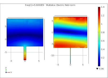
The results before and after optimization can be seen in the Fig. 1

Fig. 1 Electric field on the patch before and after optimization

.

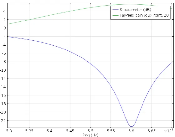
Fig. 2 Simulations of dependence antenna gain and frequency parameter S11on the reference zone before optimization.

Fig. 2 Simulations of dependence antenna gain and frequency parameter S11on the reference zone after optimization.

After optimization, the antenna gain was increased from 1-1,5dB to 1,5-5dB. The parameter S11 has standard value with the minimum of -23dB.

R

EFERENCES

[1] Chang, Kai. RF and microwave wireless systems. 1. New York: Wiley, 2000. ISBN 0471351997.

[2] Milligan, Thomas A. Modern antenna design. 2nd ed. Hoboken, N.J.: Wiley-Interscience, c2005, xvi, 614 p. ISBN 04-714-5776-0. [3] Vícepásmová flíčková anténa Multi-band spot antenna: Číslo přihlášky: 2005-816. Praha Úřad průmyslového vlastnictví 2008.

Přihlášeno 20051227. Uděleno 20081112.

[4] Lagarias, J.C., Reeds, J.A., Wright, M.H., Wright, P.: Convergence properties of the Nelder -Mead simplex algorithm in low dimensions. SIAM J. Optim. 9, 112–147 (1998)

[5] Nelder, J.A., Mead, R.: A simplex method for function minimization. Comput. J. 7, 308–313 (1965)