Objective Assessment of Machine Learning Algorithms for Speech Enhancement in Hearing Aids

Western University Western University

Scholarship@Western

Scholarship@Western

Electronic Thesis and Dissertation Repository

12-10-2018 10:30 AM

Objective Assessment of Machine Learning Algorithms for

Objective Assessment of Machine Learning Algorithms for

Speech Enhancement in Hearing Aids

Speech Enhancement in Hearing Aids

Krishnan Parameswaran The University of Western Ontario

Supervisor Parsa Vijay

The University of Western Ontario

Graduate Program in Electrical and Computer Engineering

A thesis submitted in partial fulfillment of the requirements for the degree in Master of Engineering Science

© Krishnan Parameswaran 2018

Follow this and additional works at: https://ir.lib.uwo.ca/etd

Part of the Signal Processing Commons

Recommended Citation Recommended Citation

Parameswaran, Krishnan, "Objective Assessment of Machine Learning Algorithms for Speech Enhancement in Hearing Aids" (2018). Electronic Thesis and Dissertation Repository. 5904.

https://ir.lib.uwo.ca/etd/5904

This Dissertation/Thesis is brought to you for free and open access by Scholarship@Western. It has been accepted for inclusion in Electronic Thesis and Dissertation Repository by an authorized administrator of

ii

Abstract

Speech enhancement in assistive hearing devices has been an area of research for many

decades. Noise reduction is particularly challenging because of the wide variety of noise sources

and the non-stationarity of speech and noise. Digital signal processing (DSP) algorithms deployed

in modern hearing aids for noise reduction rely on certain assumptions on the statistical properties

of undesired signals. This could be disadvantageous in accurate estimation of different noise types,

which subsequently leads to suboptimal noise reduction. In this research, a relatively unexplored

technique based on deep learning, i.e. Recurrent Neural Network (RNN), is used to perform noise

reduction and dereverberation for assisting hearing-impaired listeners. For noise reduction, the

performance of the deep learning model was evaluated objectively and compared with that of open

Master Hearing Aid (openMHA), a conventional signal processing based framework, and a Deep

Neural Network (DNN) based model. It was found that the RNN model can suppress noise and

improve speech understanding better than the conventional hearing aid noise reduction algorithm

and the DNN model. The same RNN model was shown to reduce reverberation components with

proper training. A real-time implementation of the deep learning model is also discussed.

Keywords

Machine learning, Deep learning, Digital signal processing, Hearing aid, Recurrent Neural

iii

Acknowledgments

I would like to thank my supervisor, Associate Professor, Dr. Vijay Parsa, Principal

Investigator, National Centre for Audiology, for guiding me through my research work during the

last two years. I would also like to thank the faculty members of National Centre for Audiology

for their direct/indirect support during my research. I shall extend my gratitude to Ontario

Research Fund group which offered financial support for the project.

I take this opportunity to thank my peers and friends who supported me and motivated me

throughout my research period. Lastly, I express my indebtedness to my family members for

iv

Table of Contents

Abstract……….. ii

Acknowledgments………... iii

Table of Contents………... iv

List of Tables………. vii

List of Figures………..…. viii

List of Acronyms………..……… vii i Chapter 1……… 1

1 Introduction………... 1

1.1 Background……….. 1

1.2 Brief history of hearing aids……….…………... 2

1.3 Signal processing in hearing aids……….……… 4

1.4 Introduction to machine learning……….……… 5

1.5 Problem statement and contributions………... 6

1.6 Thesis outline……….……. 6

Chapter 2……….. . 7

2 Conventional signal processing algorithms………. 7

2.1 Digital Signal Processing over the years……….……… 7

2.2 Signal Processing in hearing aids……...……….……… 8

2.3 Audibility………. 10

2.4 Sound cleaning………. 11

v

3 Machine learning in hearing aids………….………18

3.1 Types of machine learning……….………18

3.2 Artificial Neural Networks (ANNs)……….……… 19

3.2.1 Activation function……….……… 20

3.2.2 Feedforward neural network……….. 21

3.3Learning process in neural networks……….... 22

3.3.1 Forward propagation……….. 22

3.3.2 Back propagation………....………… 23

3.4Regularization………... 24

3.5 Recurrent Neural Network……… 25

3.5.1 Back propagation through time……….. 26

3.5.2 Vanishing gradient problem………... 27

3.5.3 Long Short-Term memory………. 28

3.5.4 Gated Recurrent Unit………. 31

Chapter 4………. 32

4 Implementation ……….. 32

4.1 Feature extraction……….. 33

4.2 Neural Network architecture………. 36

4.3 Training………....………. 37

4.31. Loss function……… 38

4.3.2 Optimization………. 38

4.4 Database………. 40

4.5 Pretrained RNN model………... 41

4.6 Evaluation metrics……….. 42

4.6.1 Short-Time Objective Intelligibility (STOI) measure………... 42

4.6.2 Hearing Aid Speech Perception Index (HASPI)………... 44

4.6.3 Hearing Aid Speech Quality Index (HASQI)………... 46

vi

4.7.1 Band energy………. 48

4.7.2 Band correlation……….. 49

4.7.3 Interpolated band gain………. 49

Chapter 5………... 51

5 Experimental results………... 51

5.1 Open Master Hearing Aid………... 51

5.2 DNN-based speech enhancement………... 54

5.3 Bark filter bank-based speech enhancement……… 56

5.3.1 Scaling of input waveforms……… 57

5.3.2 Different SNRs………57

5.3.3 Acoustic context………... 58

5.3.4 Final configuration………... 59

5.4 Dereverberation………...………. 61

5.4.1 Convolution and addition……… 63

5.4.2 Acoustic context………... 64

5.4.3 Comparison of results……….... 65

5.5 Portable implementation………...………… 67

Chapter 6……….... 68

6 Conclusion………. 68

6.1Summary………... 68

6.2 Future work………... 69

References……….. 70

vii

List of Tables

Table 4.1: Gammatone frequencies………. 48

Table 5.1: Intelligibility (HASPI) index values - Speech with noise for different

models………. 59

Table 5.2: Quality (HASPI) index values - Speech with noise for different models…….. 60

Table 5.3: Intelligibility (HASPI) index values - Speech with reverberation for different

models………. 65

Table 5.4: Quality (HASQI) index values - Speech with reverberation for different

viii

List of Figures

Figure 2.1: Signal Processing in hearing aids……….. 8

Figure 2.2: A comparison of performance of different spectral subtraction methods……. 14

Figure 3.1: Artificial neuron……… 20

Figure 3.2: a) sigmoid activation b) ReLU activation function………20

Figure 3.3: Multilayer Perceptron (MLP)……… 22

Figure 3.4: Recurrent Neural Network……… 26

Figure 3.5: RNN unrolled in time……… 27

Figure 3.6: Mathematical model of RNNs……….. 29

Figure 3.7: Mathematical model of LSTMs……… 30

Figure 3.8: Operations………. 30

Figure 3.9: Gated Recurrent Unit……… 31

Figure 4.1: Noise reduction scheme……… 32

Figure 4.2: Speech enhancement using RNN model………34

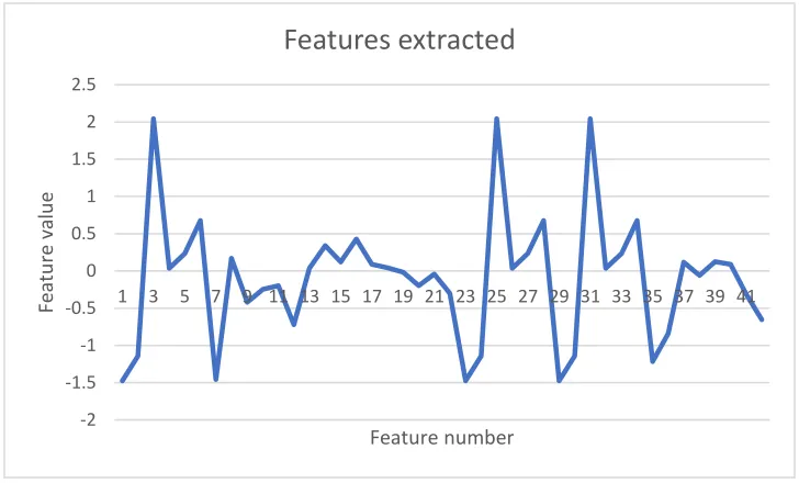
Figure 4.3: Features from an audio frame………35

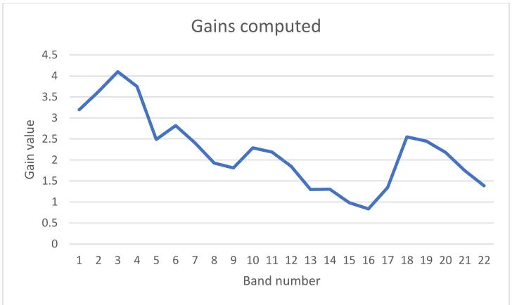
Figure 4.4: Gains computed for an audio frame during Bark frequency analysis…………35

Figure 4.5: RNN model………37

ix

Figure 4.7: Spectogram……… 41

Figure 4.8: STOI model……….. 43

Figure 4.9: Comparison of STOI values between noisy speech and the output of pretrained RNN model at SNRs -3dB, 0dB and 3dB……… 43

Figure 4.10:HASPI model………44

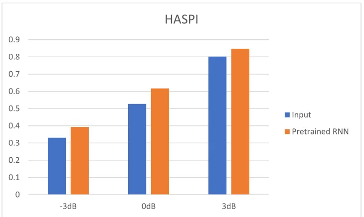
Figure 4.11: Comparison of HASPI values between noisy speech and the output of pretrained RNN model at SNRs -3dB, 0dB and 3dB………. 45

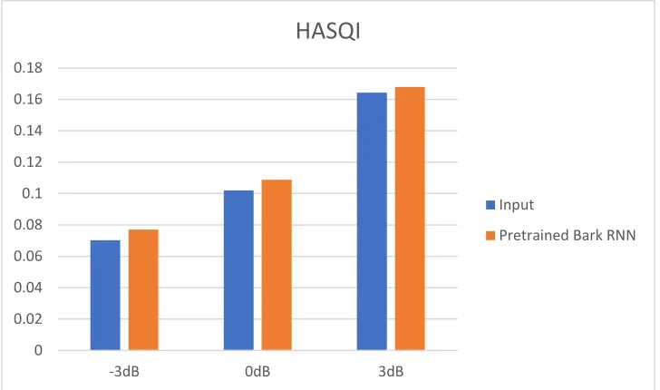
Figure 4.12: Comparison of HASPI values between noisy speech and the output of pretrained RNN model at SNRs -3dB, 0dB and 3dB……… 47

Figure 4.13: Comparison of HASPI values between input and output of RNN trained with Gammatone features at SNRs -3dB, 0dB and 3dB……… 50

Figure 5.1: OpenMHA framework………. 51

Figure 5.2: Waveform representation of a) Input noisy speech b) Output of pretrained RNN c) Output of MHANR algorithm……… 53

Figure 5.3: HASPI comparison between pretrained RNN and MHANR……….. 54

Figure 5.4: Speech enhancement by DNN model………. 55

Figure 5.5: Waveform representation of a) input noisy speech b) output of pretrained RNN model c) output of RBM-based DNN model………. 55

Figure 5.6: HASPI comparison between pretrained RNN and DNN models………56

Figure 5.7: HASPI values for different scaling configurations………. 57

Figure 5.8: HASPI values for different SNR configurations………. 58

x

Figure 5.10: Graphical representation of HASPI values - Speech with multitalker

babble for different models……….59

Figure 5.11: Graphical representation of HASQI values - Speech with multitalker

babble for different models……… 60

Figure 5.12: Spectrogram of a) Noisy input at 0dB SNR, b) Output from pretrained

RNN model, c) OpenMHA output RBM model output, e) Output from

trained GT RNN model and f) Output from trained Bark RNN model………61

Figure 5.13: Measurement of room impulse response calculation……….. 62

Figure 5.14: a) Speech with impulse response of Aula Carolina b) Speech with lecture

c) Speech with booth d) Speech with office………62

Figure 5.15: HASQI values with different methods for convolution……….. 62

Figure 5.16: HASQI values for different window size……… 63

Figure 5.17: Graphical representation of HASPI values - Speech with reverberation

for different models………. 64

Figure 5.18: a) Input reverberating (office) speech, b) Output of pretrained,

RNN model c) Output of RNN model trained with noise, d) Output of

RNN model trained with reverberated speech……… 65

Figure 5.19: Graphical representation of HASQI values - Speech with reverberation

xi

List of Acronyms

HA Hearing Aid

DSP Digital Signal Processing

dB Decibels

SNR Signal to Noise Ratio

CMOS Complementary Metal Oxide Semiconductor

ML Machine Learning

RNN Recurrent Neural Network

VLSI Very Large Scale Integrated

ASIC Application Specific Integration Circuit

ADC Analog-to-Digital Converter

IIR Infinite Impulse Response

FIR Finite Impulse Response

FFT Fast Fourier Transform

IFFT Inverse Fast Fourier Transform

SPL Sound Pressure Level

ILD Interaural Level Difference

BTE Behind-The-Ear

BSS Basic Spectral Subtraction

SOS Spectral Over Subtraction

NSS Non-Linear Spectral Subtraction

MBSS Multi-Band Spectral Subtraction

WF Weiner Filter

WGN White Gaussian Noise

PSD Power Spectral Density

ISS Iterative Spectral Subtraction

SSPP Spectral Subtraction Based on Perceptual Properties

DNR Digital Noise Reduction

DNN Deep Neural Network

xii

ANN Artificial Neural Network

ReLU Rectified Linear Unit

DAG Directed Acyclic Graph

MLP Multi-Layer Perception

MSE Mean Squared Error

MAE Mean Absolute Error

BP Back Propagation

BPTT Back Propagation Through Time

LSTM Long Short-Term Memory

GRU Gated Recurrent Unit

VAD Voice Activity Detector

DCT Discrete Cosine Transform

BFCC Bark Frequency Cepstral Coefficients

HINT Hearing In Noise Test

STOI Short-Time Objective Intelligibility

OIM Objective Intelligibility Measure

AI Articulation Index

SII Speech Intelligibility Index

STI Speech Transmission Index

CSII Coherence-Based Speech Intelligibility Index

ITFS Ideal Time Frequency Segregation

TF Time Frequency

DFT Discrete Fourier Transform

HASPI Hearing Aid Speech Perception Index

TFS Temporal Fine Structure

IBM Ideal Binary Mask

OHC Outer Hair Cell

IHC Inner Hair Cell

MFCC Mel-Frequency Cepstral Coefficients

BM Basilar Membrane

xiii

CC Cepstral Correlation

GT Gammatone

ERB Equivalent Rectangular Bandwidth

MHA Master Hearing Aid

LPC Linear Predictive Coding

NLMS Normalised Least Mean Squared

MHANR Master Hearing Aid Noise Reduction

CLA Command line Application

IO Input-Output

JACK Jack Audio Connection Kit

TCP/IP Transmission Control Protocol/Internet Protocol

SCNR Single Channel Noise Reduction

RBM Restricted Boltzmann Machine

CD Contrastive Divergence

MMSE Minimum Mean Squared Error

AIR Aachen Impulse Response

OS Operating System

1

Chapter 1

1. Introduction

This chapter deals with the background, a brief history of hearing aids (HAs), conventional

signal processingalgorithms in hearing aids, machine learning in hearing aids and thesis outline.

1.1 Background

Individuals who are unable to listen clearly like those with normal hearing ability i.e.

hearing thresholds (sound level below which a person’s ear is unable to detect any sound) of 25

dB (decibels) or better in both the ears are known to be suffering from hearing impairment [1]. In

other terms, hearing loss is characterized by an increase in hearing, threshold for a sound

frequency. It implies that the hearing sensitivity decreases, eventually, making it difficult for the

listener to detect soft sounds. The magnitude of hearing loss can range from mild to moderate,

severe, or profound, affecting either a single ear or both the ears thereby making it difficult to hear

conversational speech or loud sounds. The reasons for loss of hearing or deafness may be

congenital or acquired.

Statistics reveal that approximately 466 million individuals around the world have

problems of disabling healing loss of which 34 million are reported to be children. Disabling

hearing loss indicates hearing loss greater than 40 decibels (dB) in the better hearing ear in adults

and a hearing loss greater than 30 dB in the better hearing ear in children. Studies reveal that by

the year 2050 roughly nine hundred million individuals (one in every ten people) are likely to

suffer from disabling hearing loss [1].

The exposure of the younger generation aged between 12 and 35 years, to loud noise in

recreational settings have posed a risk of hearing loss to about 1.1 billion people in this cohort.

The annual world-wide cost of unaddressed hearing impairment is estimated to be US$750 billion

[1]. Preventing, identifying and addressing hearing impairment issues are cost-effective, bring

huge benefit to people. Majority of these hearing-impaired people require custom assistive hearing

devices.

The intelligibility of human speech is quite significant in hearing and communication. It is

2

characteristics, conditions in communication and capacity of information as well as the ability to

gather information from a specific context, mimics and gesture determine the quality and

intelligibility of speech [2]. Intelligibility can be better understood by discussing the distinction

between real and recorded speech. In a real conversation, individuals will be able to

identify/distinguish the sounds in the background and focus on the speech of the person

conversing, thus filtering the desired information from the audio environment. This helps to

significantly increase the speech intelligibility and comprehension although the communication

may happen in a noisy environment [2].

The environment in which speech signals are transmitted are typically noisy in real-time

situations. Persons with normal hearing may understand speech in a moderately noisy environment

since speech is an extremely redundant signal [3]. Therefore, even if part of the signal is masked

by noise, the unmasked part may still allow the speech segments to be intelligible for effective

communication. Comparatively, there is reduced redundancy in speech signal for individuals

suffering from hearing impairment because the either the speech is partially audible or is severely

distorted. Background noise that masks even a small portion of the remaining speech signal will

degrade intelligibility significantly. Thus, people with hearing loss have a greater difficulty in

understanding speech in a noisy environment than the people with normal hearing [3].

The noise potential for masking speech is expressed by the Signal-Noise Ratio (SNR)

which is the ratio of the power of speech signal to the power of noise, when both are presented

concurrently. Lower the value, bigger is the loss in understanding of speech for both normal

hearing and hearing impaired[4]. Consequently, as the SNR increases, the speech intelligibility

improves significantly.

1.2 A brief history of hearing aids

Hearing aids are small electronic devices that amplifies sound and makes it easier to

understand speech. They are designed in a way that they can capture sound waves using a very

small microphone, modify softer sounds into audible sounds, and finally pass the same to the ear

by means of a tiny speaker, enabling individuals with hearing disability to perceive sounds again,

and enhance their ability to hear. Thus, it can acquire, process and feedback acoustic signal in real

time in noisy conditions [2]. In the modern day, with the help of microchips, hearing aids are not

3

The invention of hearing aids is centred on no single person. Though there are no recorded

dates, it is believed that ear horns have existed in every civilization for thousands of years since

humans first created carved objects. Giovanni Battista Porta was most likely the first to describe

ear trumpet, a metal version of the ear horn, around 1588 [5]. The 17th century saw the growth of

speaking tubes as assistive hearing devices until pre-electric horns and trumpets became popular.

In the 1800s the introduction of decorative and functional hearing aids which could be

concealed and made less obvious, addressed the concerns regarding public perception about

hearing aids [5]. Finally, in the nineteenth century the idea of electrically-powered hearing aid

instruments was introduced which consisted a battery box, earpiece and microphone, made of

carbon dust which was to be refined later.

The first electronic hearing aids were devised after the invention of the telephone (the

technology within which increased how acoustic signal could be altered) and microphone in the

1870s and 1880s. In 1898 Miller Reese Hutchison created the first electric hearing aid and named

it Akouphone [6]. The use of carbon transmitter assisted in amplifying the sound by taking a weak

signal and making the same stronger with the help of electric current.

The invention of microprocessor led to the miniaturization of hearing aids. In 1987, the

first commercial digital hearing aids was invented. Until then, the hearing aids were analog in

nature. In analog hearing aids, incoming noise are dealt with by taking electrical sound waves

emerging from the microphone, amplifying the same ‘as is’ and transmitting it to the ear while

digital hearing aids transforms soundwaves from a microphone into digital binary code which is

in turn altered by a microchip within the hearing aids prior to transforming back into analog signals

and delivering to the speaker [7].

The functionalities of both analog and digital hearing aids are basically similar i.e taking

sounds to amplify them so that they can assist with better hear. Both analog and digital hearing

aids are programmable, whereby the microchips within can be customised to improve the sound

quality and matched with the individual user. At the same time, they can be customised to develop

4

quiet environment and can be readjusted while in a noisy restaurant and further readjusted in large

auditoriums.

Compared to analog hearing aids, digital hearing aids contain additional features and

flexibility which are perceived to be user-configurable as it has the ability to modify sound in

digital form. For example, digital hearing devices offer numerous channels and memories,

providing advantage of being able to save more location-specific profiles. Additionally, digital

hearing aids possess the capability to decrease surrounding noise automatically, eliminate

feedback or whistling, or the capability to favour human voices over any other noise.

1.3 Signal processing in hearing aids

Digital Signal Processing (DSP) is a relatively recent technique that involves the sampling

of an analog signal and the processing of these samples in digital form. This processing can be

accomplished using standard digital integrated circuit technologies such as complimentary metal

oxide semiconductor (CMOS), which is space and energy efficient. The digital processing of

speech is a mature technology and a wide range of algorithms is available for filtering,

compression, noise reduction, dereverberation, feedback reduction and special effects as well as

coding for bandwidth reduction. Many of these techniques would prove beneficial to the hearing

impaired if tailored correctly to their needs and implemented in a hearing aid [8].

Signal processing research on digital hearing aids encompasses signal acquisition,

amplification, transmission, measurement, filtering, parameter estimation, separation, detection,

enhancement, modeling, and classification [9]. They can be broadly categorised into four areas.

The first area adopts advanced signal processing methods to characterize and compensate for

hearing loss like loudness and frequency selectivity loss. The second area focuses on effective

target signal improvement and reducing noise, including adaptive microphone array technologies,

spectral subtraction algorithms, and blind source separation methods. The third area consists of

practical usage of hearing aids to address problems like flexibility, convenience, feedback

cancellation, and artifact reduction. Finally, the fourth area concentrates on developing hearing aid

technology into devices, the functions of which can also be used for hand phones and music players

[9]. Here the focus is mainly placed on problems like echo cancellation, bone conductive

5

necessities, computational speed, consumption of power and other pragmatic issues, the

advancement and application of signal processing methods in digital hearing aids have faced

numerous challenges in the last decade [9].

1.4 Introduction to machine learning

Machine learning is a technique of analysing data, which helps to automate building of

analytical models. It is that branch of artificial intelligence, which adopts the idea that data can be

learnt effectively from the systems, patterns can be identified, and decisions can be made with

little human involvement. This field of computer science uses statistical methods and provides

computer systems a learning ability to improve performance, gradually on specific tasks, either

with or without explicitly programming the data.

Machine learning has applications in various areas such as image recognition (face

detection and recognition in Facebook), speech recognition (as in Siri in Apple phones and Alexa

for home automation), medical diagnosis (prediction of disease progression), product

recommendation (as in Amazon, Netflix or Youtube websites), basket analysis (learning

association between products people buy), classification and prediction of potential customer

behaviours in terms of loan repayment in banks, real-time information extraction from web pages,

data security (predicting which files are malware), fraud detection (in PayPal), traffic and route

recommendations (as in Google Maps) etc.

While implementing conventional signal processing algorithms in digital hearing aids, the

speech characteristics need to be learnt, analysed and then hard coded to segregate speech in audio

segments. Similarly, the types of noise and various environments that the hearing-impaired

listeners are subjected to, must be known during design to be able to program the noise

characteristics into the hearing aids. Recently, machine-learning approaches to enhancement of

speech have been promising in refining speech intelligibility for people with hearing impairment.

A machine learning model understands the underlying details and learns to differentiate speech

from noise when trained with features of speech and noise separately. The recent researches also

indicate that deep learning can be used for automatic speech recognition where latency is not

important [18]. This project focuses on speech enhancement using a combination of signal

6

1.5 Problem statement and contributions

Conventional noise reduction techniques in modern hearing aids work well with stationary

noise. They may also provide improvement in SNR. However, the improvement in SNR does not

necessarily enhance speech intelligibility as per behavioural studies. The conventional

methodologies have limitations processing non-stationary noise. Recently, deep learning-based

models have been found to perform better than conventional algorithms for hearing aid

applications. This thesis focuses on training and implementation of a deep neural network for the

purposes of noise reduction and dereverberation, evaluation of its performance using objective

predictors of speech intelligibility and quality and real-time implementation of the algorithm in a

portable computing platform.

1.6 Thesis outline

This thesis is organized in chapters that discuss conventional signal processing algorithms

in a bit more detail (chapter 2), Machine Learning (ML) and its speech applications so far (chapter

3), the implementation of speech enhancement algorithm, database used to evaluate it, the

objective metric and comparison between Gammatone and Bark filters (chapter 4), results from

the objective assessment of pretrained and trained Bark RNN and their comparison with a couple

7

Chapter 2

2 Conventional signal processing algorithms

Signal processing in hearing aids has come a long way over the past few decades. This

chapter briefly discusses the advancement in digital signal processing (DSP) over the past few

decades, outlines the various DSP algorithms incorporated into hearing aids, and finally focuses

on the conventional noise reduction DSP algorithms and their effectiveness in enhancing speech

perception by hearing impaired listeners.

2.1 DSP over the years

The world is becoming more and more digital in our daily activities since the invention of

integrated circuits. Not only did the size of microelectronics shrink, but the computational power of the microelectronic systems doubled almost every two years. This follows the “Moore’s law of microelectronics” which led to a remarkable influence on the technology within hearing aids. An

all-digital hearing aid was reported to be developed in the 1980s [10]. Researchers created several

prototype hearing aids with the help of customised DSP chips using less power as well as very

large scale integrated (VLSI) chip technology. These hearing aids were put to use for research on

individuals with hearing-impairment. Now, most of the commercially available hearing aids are

digital. Modern hearing aids have become intelligent systems providing a wide variety of

algorithms for specific and diverse hearing and communication challenges of users in various

acoustic environments [10].

Numerous hearing aids, in the modern times, comprise application-specific integrated

circuits (ASICs) as well as reprogrammable DSP cores and microcontroller cores providing

advantages of flexible reuse of the microelectronics for different signal processing algorithms.

There has been significant improvement in the performance of digital hearing aids during the last

two decades [10]. The objectives of hearing aids have been upgraded to improve quality of sound

by reducing the artifacts and providing more natural sound output, in addition to improving speech

intelligibility. These requirements must be met in dynamically changing listening environments in

everyday life situations.

Newer DSP platforms provide computational abilities to implement advance functions like

8

where there has been a huge improvement is in systems integration [10]. Adaptive algorithms

could sometimes counteract each other, just like algorithms for noise-cancellation and acoustic

feedback controlling algorithms are likely to decrease gain and work in opposition to amplification

schemes. These effects are taken into consideration during design, implementation as well as in

choice of parameters for signal processing algorithms. A more detailed description of individual

DSP algorithms within hearing aids is given next.

2.2 Signal processing in hearing aids

The types of hearing loss are so diverse that each of them needs custom prescriptions. One

listener may need frequency-dependent gain, the other may need level-dependent and the third

listener may need a combination of both. Thus, technology in hearing aids must be flexible enough

to be able to meet revised requirements and digital hearing aid is the solution available today.

Figure 2.1 provides a framework of signal processing algorithms in digital hearing aids of modern

times. The signals from the environment that come to listener’s ear are picked up by one or more

omnidirectional microphones. These signals would be analog in nature. Hearing aids in the early

stages used to process analog signals only which means amplification of input in simple terms.

This may not help the hearing-impaired listeners much and in fact amplification could just cause

distress.

Figure 2.1: Signal processing in hearing aids Sound Pickup Sound cleaning wireless audio

FFT

IFFT Environment classification

Signal output output Acoustic Mechanic Electric IFFT Analysis filter bank Gain calculation (incl. amplitude compression) Synthesis filter bank Environment detection Adaptive beam former Pinna simulation MIC matching steering Noise reduction

• Stationary noise

• Impulsive noise

9

The analog signal (sound waves) is converted to electrical signal by the vibration of

diaphragm in microphones which is caused by the changes in air pressure. This electrical signal is

then sampled and digitized using an Analog-to-Digital Converter (ADC), which usually provides

a usable audio bandwidth of 8 to 16kHz. The resultant discrete time signal may be analyzed

spectrally either in frequency domain or in time domain depending on the signal processing

algorithm used in the device[10]. Either of the methods will involve trade-offs in time-frequency

resolution. The hearing devices these days are expected to have a delay no more than 10-12ms to avoid incongruity between the speaker’s lip movement, echo and the audio signal [10]. The

spectral resolution is dependent on frequencies with bandwidth proportional to center frequency.

The time domain analysis of speech signals can be done using a bank of infinite impulse

response (IIR) filters as: Signal from microphone → Filter bank (Combination of low pass, band

pass and high pass filters) → Sound cleaning → Loudness adjustment → Recombination of signals

into single output. Each of the filters in filter bank may allow or stop a specific range of frequencies

that form a band. The channel width increases with center frequency with more frequency

resolution at lower frequencies. IIR filters require much lesser computation to achieve desired filter

slopes when compared to FIR filters. However, a cautious design is required to evade the artifacts

that may be produced otherwise. It is recommended to process a block of samples instead of

processing each sample when it comes for computational efficiency [10].

The analysis in frequency domain is done by taking Fourier transform of the signal: Store

specific number of samples in a buffer → Multiply the values with a window function (to avoid

discontinuities at the edges) → Apply Fourier transform (FFT) → Sound cleaning → Loudness

adjustment → Inverse FFT → Output synthesis [10].

Hybrid analysis systems combine the time domain online processing with frequency

domain offline processing. The signal collected by microphone is processed first in time domain

up to sound cleaning, which is summed across channels before passing it on to the filter bank in

frequency domain. Such systems join lower quantization sound as well as the time domain filter

distortion with the higher frequency resolution of FFT systems. At the same time there is little

need to smoothen the gain across frequency or have large temporal overlap between consecutive

blocks. Time-frequency analysis schemes form the basis for different adaptive algorithms though

10

The signal processing algorithms are broadly classified into three types based on their

functionality:

1) Frequency and level-dependent gain application to provide a satisfactory volume for

the respective hearing profile (usually audiogram)

2) Sound cleaning by removal of stationary and non-stationary noises and reducing

acoustic feedback through the use of various algorithms for noise reduction.

3) Environment classification for automatic adjustment of hearing aid settings to choose

suitable signal processing algorithm for a given condition

No single algorithm may provide optimal performance in all these aspects. Though

different manufacturers may have or come up with entirely different signal processing strategies

and solutions the underlying class of these strategies remain same with premises and scope clearly

defined for each of these solutions.

2.3 Audibility

There are a couple of important strategies to restore audibility. Most people suffering from

sensorineural hearing impairment endure loudness recruitment, a phenomenon which causes the

loudness to grow rapidly for any sound above the absolute threshold. The gain should reduce when

input levels increase to compensate this effect, which means the input-output function is

compressive and the process by which we achieve it is called multichannel compression. For lower

inputs, up to about 40 dB SPL, the gain is kept constant. The applied gain decreases with further

increase up to 100 dB SPL which compensates loudness recruitment and the compression ratio is

made infinite beyond 100 dB SPL for limiting [10]. The compression algorithms can be

slow-acting (like in Adaptive Dynamic Range Optimization) based on input sound level which will help

maintain signals for localization of sound based on Interaural Level Differences (ILD) or

fast-acting which will have comparatively shorter attacks and release times and are able to make

loudness perception level closer to normal.

Many a times it is quite tough to restore audibility at high frequencies for individuals

suffering from extreme hearing loss. Applying gains at these frequencies could cause acoustic

feedback or loudness discomfort, especially when they have narrow dynamic range. Frequency

lowering is an alternative approach in such situations. This would be perceptually beneficial

11

into three categories: a) frequency transposition – a block of higher frequency component is shifted

downward to a frequency in destination band, b) frequency compression or frequency division –

frequency components up to a frequency stay unaffected and the components above are shifted

downward with a lower slope and c) spectral envelope warping - lowering of part of the spectral

envelope, keeping the spectral components unchanged.

2.4 Sound cleaning

It is important to note that restoring audibility alone will not suffice for speech perception

in acoustically challenging environments. It is indeed challenging for hearing-impaired people to

understand speech (intelligibility) in noisy environments. Though reducing noise may sound an

easier task, this has been a prime area of focus since the invention of digital hearing aids. There

are so very divergent types of speech and background noise to deal with. What makes it more

difficult is the constantly changing speech and noise in realistic sound scenarios. The target speech

differs due to the characteristics of speaker, vocal effort, distance and orientation of the speaker,

the amount of reverberation in the listening environment and the presence/absence of visual cues.

Due to this variability, a single algorithm for optimal noise reduction is not available.

The most successful approach for noise reduction uses directional microphone, that can

help when there is a spatial separation of target speech from source of the noise. Hearing aids using

this technique will have two omnidirectional microphones – one at the front and the other toward

the back side. The signal collected from one microphone is delayed and added with the other to

form a beam pattern. In this manner, the target signal from the beam’s direction will be captured

and others will be attenuated. The shape of beam pattern is constant in a static beamformer whereas

it dynamically adapts based on environment in an adaptive beamformer. When the direction of

highly interfering sound changes, the adaptive beamforming system shall adjust itself to maintain

the good suppression of the interference. The beamformer may be independently applied to various

frequency bands instead of the entire broadband signal.

Directional microphones provide 2-5 dB improvement in the threshold of speech reception

in realistic conditions [10]. Though use of these microphones is advantageous in many ways, these

may not help in understanding of speech coming from side or back like a vehicle coming from

12

microphones such as in the Behind-The-Ear (BTE) hearing aids, far from the pinna may also affect

their directivity.

Binaural beamformer is a technique combining the four microphones of two bilaterally

worn hearing aids that forms a four-microphone directional system. The outputs of two

microphones on both sides are initially combined before exchanging over a wireless link with the

hearing aid on the other side. Thus, the ipsilateral and contralateral signals in each hearing aid are

combined using a frequency dependent weighting function to create binaural directivity pattern,

which is narrower than the monoaural one. This static beamformer can be made adaptive by

combining the resulting signal in one hearing aid with the current spatiotemporal distribution of

undesired signals. Researches earlier have demonstrated the way this approach can enhance speech

intelligibility while reducing the effort made to hear.

The above two approaches assume that source of speech is directly at the front side of the

listener. However, this is not the case in many of the communication scenarios, just like the target

could be on the side while driving. A solution for such a situation is to pick up signal from the ear

that is ipsilateral (better ear) to the target and transmit the same to the contralateral side. This will

allow both the ears to receive a reasonably clean representation of the target.

In situations where speech and noise are spatially co-located, or in small-size custom

hearing aids which preclude the placement of two microphones due to size restrictions, additional

strategy is required for noise reduction. Single microphone noise canceling algorithms are such

strategies and represent one of the most widely used techniques in digital hearing aids today. It

works on the premise that speech signal has different temporal properties than that of the

interfering sounds and that low-rate temporal fluctuations are relatively scarce in case of the

background sounds. These temporal fluctuations in speech signal are used to estimate the SNR,

which is used in computationally efficient algorithms like spectral subtraction, harmonic

extraction, and Wiener filtering techniques to reduce interference. These algorithms are briefly

described next.

One of the initial noise reduction algorithms that was first proposed for single channel

speech improvement was spectral subtraction (BSS) [11]. It is a technique to restore power or the

magnitude spectrum observed signals in additive noise, by subtracting the estimated average noise

13

from the periods when there is no signal while the noise alone exists. In this manner, the estimation

of noise spectrum is made when there are pauses in speech and is deducted from the spectrum

when the speech is noisy. While doing so, an assumption is made that the noise is not correlated

with speech and that the noise is additive in nature. Many variants of spectral subtraction are

present, and the principle for all the variants is to estimate short time speech spectral magnitude

by deducting sound from noisy speech or by multiplying the noisy spectrum with gain functions

and combine with the phase of noisy speech.

Spectral over-subtraction (SOS) introduced two extra parameters such as over-subtraction

factor and noise spectral floor in basic spectral subtraction method to reduce remnant noise

(processing distortion), which is one of the two drawbacks of BSS, the other being narrow band

musical noise [11]. The over-subtraction factor restricts the quantum of noise power spectrum

subtracted from the noisy speech power spectrum in each frame. The spectral floor parameter helps

to dissuade the ensuing spectrum from dipping beyond a pre-determined minimum level instead

of setting to zero (spectral floor). This implementation considers that the speech spectrum is

affected by noise evenly and the subtraction factor subtracts an over-estimate of noise from noisy

spectrum. In order to draw a balance between the surrounding noise and remnant noise elimination,

numerous combinations of over-subtraction factor α, and spectral floor parameter β provides a

trade-off between the quantity of residual noise in the background and the extent of perceived

remnant noise. Because noise is perceived to influence speech spectrum equally and that the

over-subtraction feature is constant across frequencies, the enhanced speech may be distorted.

In reality, noise is colored and influences speech signal in a different way throughout the

spectrum and subtraction factor is expected to be frequency dependent to explain various types of

noise. The non-linear spectral subtraction (NSS) idea, extends this ability by forcing the

dependency of the over-subtraction factor frequency while the subtraction process remains

non-linear. Bigger values are deducted at frequencies with low SNR levels, and lesser values are

deducted at frequencies with high SNR levels giving better flexibility for compensation of errors

in the estimation of noise energy in various frequency bins [11].

Multi-band spectral subtraction (MBSS) groups frequencies into bands and multiple bands

14

random in nature, enhancement in MBSS algorithm is required for the reduction of WGN. The

MBSS algorithm usually performs better than other subtractive-type algorithms.

In a Wiener filter (WF) design it is assumed that speech and noise are not correlated [11].

They are considered to be in normal distribution and this filter aims to reduce the mean squared

error criterion. The gain function of WF is fixed at all frequencies and it requires power spectral

density (PSD) of clean signal and noise for filtering, which are the main drawbacks of WF. It is

not possible to apply non-causal WF directly in order to estimate clean speech since it is not

possible to assume that speech is stationary. An adaptive WF implementation decreases each

component of frequency by a certain amount that depends on the power of noise at that frequency.

The gain function in WF is calculated using power spectrum of noisy speech, rather than

clean speech which will degrade its accuracy. An iterative algorithm is used to solve this problem.

In the iterative spectral subtraction (ISS) algorithm, the improved speech output is taken to be the

input for following iteration and consequently for spectral subtraction, the remnant noise is

re-estimated in every iteration. Therefore, a larger number of iterations will provide a better enhanced

speech when compared to WF.

Figure 2.2: A comparison of performance of different spectral subtraction methods [11]

The use of fixed subtraction parameter is one of the major drawbacks of spectral

subtraction while the noise spectrum in real time is changing constantly. Although MBSS will

allow the adaptation of parameters, the remnant noise is not completely suppressed especially at

15

properties of spectral subtraction[11]. By incorporating the masking properties of human auditory

system into enhancement process, it is possible to attenuate components of noise that were

previously inaudible as a result of masking. Based on the masking properties, the subtraction

parameters are adapted in the algorithm. Through the calculation of noise masking threshold,

masking properties are modelled.

The spectral subtraction effectiveness is highly depending on estimation of accurate noise

that is mostly a tough task. Since the power spectrum and magnitude are non-negative variables,

the negative estimates of these variables, if any, must be mapped into a non-negative value. The

distribution of the restored signal is distorted by this nonlinear rectification method and the

distortion is more visible when the SNR reduces. Spectral subtraction that is based on perceptual

properties (SSPP) performs better in comparison to above discussed algorithms for speech

improvement. WF leads to reduced remnant noise, however, the structure of noise is musical and

speech regions, especially fricative consonants, are reduced. Such spectral subtraction can lead to

distortion of speech. Thus, using SSPP algorithm for enhanced speech is more pleasant reducing

the remnant noise with least speech distortion, if any. A comparison of various spectral subtraction

methods is demonstrated in figure 2.2, which indicates the advantage of SSPP algorithms[11].

It is important to note that difference exist among manufacturer-specific implementations

of the aforementioned spectral subtraction and Wiener filtering algorithms. Estimation of speech

and noise spectra and rules for engaging/disengaging noise are proprietary. As such, assessment

of noise reduction feature, either objectively or through subjective measurements, is of great

importance. Few studies have investigated the effectiveness of noise reduction algorithms as

implemented in commercial hearing with hearing impaired listeners. For example, Ricketts et al.

studied the effect of digital noise reduction (DNR) in hearing aids on speech recognition and

quality [12]. This subjective study with 14 adults wearing hearing aids presented that there is no

impact on speech understanding with the use of conventional noise reduction techniques although

there may be an improvement in speech quality. Another study by Bentler et al. showed that DNR

can improve listening comfort but has no effect on speech perception of even with visual cues [13].

Desjardins et al. found that speech recognition in noise score did not change much with noise

16

observed different perceptual effects among hearing aids and that none of the noise reduction

algorithms actually improved speech intelligibility while they may reduce annoyance of noise [15].

Single microphone noise canceling is usually effective for noise spectrum that hardly

changes over time and does not take into account the undesirable effects from an enclosed

environment [10]. In environments such as office, lecture rooms and big halls, the target speech

will have multiple paths from the source to listener. Apart from shortest direct path from source to

listener, the target signal could hit any part of the room (floor, ceilings or walls) and objects in the

room and reflect from them before it adds on to the direct path to listener. This process is called

reverberation and can cause severe impact on the ability to perceive speech. The performance of

beamformers depreciates when distance between target and listener increases and with increasing

reverberation. The reverberated speech can be represented as the convolution of original speech

and the impulse response of the environment. Dereverberation would need an algorithm to estimate

and segregate the parts of speech that are reflected off the objects in the reverberating environment

from the speech collected by the hearing aid.

Thus, dereverberation is a highly complex task in real-time due to its need to estimate the

constantly changing original speech target and the unknown impulse response of the room or hall.

The dereverberation approaches are generally very complicated to implement them in hearing aids

leading to time delays, which may not be acceptable for hearing aids. Lebart et al. [16] took a

simpler approach to this problem by estimating parts that are decaying over time and attenuating

them. This signal processing was done by converting the time-domain signal into frequency

domain and comparing the decay rate with respect to standard reverberation time. This method

definitely has shown improvement in quality of sound and hearing ease but does not enhance

speech intelligibility [17].

Signal processing algorithms provide a wide range of solutions to improve speech

intelligibility in adverse listening environments. However, there are limitations for every algorithm

based on environment in which it is assessed. The objective and subjective results may vary most

of the time because of the change in premises in realistic environments. Hence it is important to

specify the testing conditions and every result would be slightly or largely different from the other

17

To summarize, signal processing in hearing aids, the conventional signal processing

techniques to restore audibility and sound cleaning are discussed. Though there are many noise

reduction techniques available, the increase in SNR provided by these methods does not

necessarily improve speech intelligibility. The same is observed with dereverberation though there

are evidences of improvement in speech quality. Emerging evidence suggests that algorithms

incorporating machine learning are effective in enhancing speech understanding by

hearing-impaired listeners in noisy environments. Machine learning techniques are discussed in detail in

18

Chapter 3

3. Machine learning in hearing aids

Speech enhancement in noisy conditions has always been a challenging task for better

speech recognition and further processing, not just in hearing aids but also in all

telecommunication systems. The objective of speech enhancement is to reduce noise and to

increase intelligibility of the input noisy speech. However, the results using conventional signal

processing methodologies are not always satisfactory in terms of speech intelligibility and speech

quality, in adverse conditions. Hence there is always a need for better performing adaptive noise

reduction algorithms because of the non-stationarity of speech and noise signals.

Machine learning is that branch of artificial intelligence which has been recently found

useful in various speech recognition and natural language processing tasks. Specifically, deep

learning has the capability to learn complex patterns underlying speech data. Healy et al. used deep

neural network (DNN) to segregate speech from noise for hearing-impaired listeners [18]. This

work focused on ideal binary mask estimation with a classification approach using a Restricted

Boltzmann Machine (RBM). Chen et al. extended the work with ideal ratio mask estimation

instead using a deep neural network [19]. This chapter explains a bit about machine learning, deep

learning, artificial neural networks and their learning process.

3.1 Types of machine learning

ML algorithms are generally classified into three, based on the way the models learn.

1) Supervised learning - This algorithm includes a target or outcome variable (also known as

dependent variable) which will be predicted from a set of predictors (independent

variables). The algorithm attempts to model the relationship and dependencies between

the dependent and independent variable with the help of the given set of variables, in a way

that the output values for a new data set based on those relationship can be predicted This

training process goes on till the model is able to achieve the desired accuracy level on the

training data. Example: Regression and classification tasks

2) Unsupervised learning - In this algorithm, no target or outcome variable is available to

19

population in different groups generally uses unsupervised technique for segmenting

customers in different groups for specific intervention.

3) Semi-supervised learning – This method falls in between the above two. The cost of getting

labeled dataset is usually high and, in such situations, we obtain some labeled data along

with lots of unlabeled data for training.

4) Reinforcement learning - Here, the machine is exposed to an environment where it trains

itself repeatedly through trial and error and has to determine the ideal behaviour within the

given context to maximize performance. Q-learning, temporal difference and deep

adversarial networks are some of them.

ML can be further categorized into three based on the objective the model is trying to achieve.

1) Regression: For prediction of a continuous real number

2) Classification: For prediction of a discrete number

3) Clustering: For segmentation

Deep Learning (DL) uses different architectures of Artificial Neural Networks (ANNs) to learn

from data. These ANNs are a family of machine learning models that have taken inspiration from

human brain and the biological nervous system.

3.2 Artificial neural networks (ANNs)

An ANN is composed of neurons, which are the basic functional units inspired from

neurons in biological neural network. These neurons are interconnected to form a network of

neurons that takes in and processes a set of inputs to provide a set of outputs. The neurons (also

called as nodes) are organised in layers containing specific number of them in every layer and

connected with specific ones in another layer. Each of these connections (called edges) has a

weight that is multiplied with the conveyed value. Figure 3.1 illustrates a neuron for which 𝜃1,

𝜃2,…,𝜃N are the weights for incoming values with 𝜃0 and 1 being the weight and input representing

the bias to the neuron. The sum of weighted inputs to the neuron is passed to an activation function

that computes the output or activation of the neuron.

20

Figure 3.1: Artificial neuron

3.2.1 Activation function

An activation function is a function that transforms the input value to an output to

determine whether the neuron must be activated or not.

𝑦 = 𝑓(∑𝑁𝑖=1𝜃𝑖𝑥𝑖+ 𝜃0) (3.1)

𝑦 = 𝑓(𝜃𝑇𝑥) (3.2)

where, 𝜃 is the weight vector, x is the input vector and w0 is the bias

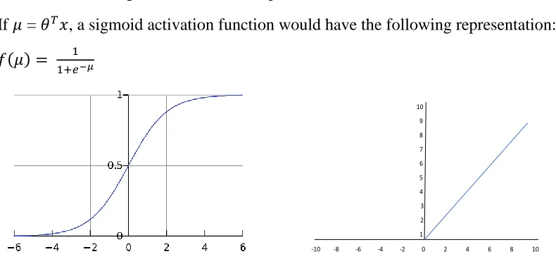
If 𝜇 = 𝜃𝑇_{𝑥, a sigmoid activation function would have the following representation:}

𝑓(𝜇) = 1

1+𝑒−𝜇 (3.3)

Figure 3.2 (from left to right) a) sigmoid activation [20] b) ReLU activation function

A Rectified Linear Unit activation (ReLU) function and a leaky ReLU are given by

𝑅𝑒𝐿𝑈: 𝑓(𝜇) = max(𝜇, 0) (3.4)

𝐿𝑒𝑎𝑘𝑦 𝑅𝑒𝐿𝑈: 𝑓(𝜇) = max(𝜇, 0) + 𝛼min (𝜇, 0) (3.5)

10 9 8 7 6 5 4 3 2 1

-10 -8 -6 -4 -2 0 2 4 6 8 10

𝑓(𝛴(∙)) 𝜃₁

𝜃₂

𝜃𝑁

𝑦 1

𝑥1

𝑥2

𝑥𝑁

21

The sigmoid activation function is linear when the weights are small and the corresponding

weighted sum is close to zero. However, it will turn non-linear as the weighted sum grows in both

the positive and negative directions as in figure 3.2a. This would result in neuron be considered on

or off as the weighted sum tends to infinity. The magnitude of bias value acts as the threshold

weighted sum that the inputs must provide to activate the neuron and contribute to output. Recent

years have seen the development of rectified non-linear activation functions like Rectified Linear

Unit (ReLU, figure 3.2b), which increases linearly for positive inputs and gives zero output for

any negative input. The drawback with ReLU is that it is not differentiable for negative inputs,

which provides no further learning. Leaky ReLU is a variant of ReLU that has a non-zero gradient

for any negative input, which is more popular for image classification tasks than conventional

ones.

Rectified non-linearity is observed to provide significant boost to the performance of object

recognition system as per [21]. [22] found that types of ReLU can provide a better model of

biological neurons than conventional hyperbolic tangent or sigmoid functions. [23] recommends

replacement of sigmoid with ReLU in feedforward neural networks.

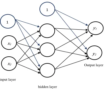
3.2.2 Feedforward neural network

Feedforward neural networks are a subclass of ANNs in which the nodes are organised in

a directed acyclic graph (DAG) from input to output. A unique type of these networks is the

multilayer perceptron (MLP) as in figure 3.3. Here the nodes are arranged in layers where

connections are provided only between neighbouring layers. The features are fed in to the first

layer which is the input layer. The output is taken from the final layer of the network termed as the

output layer. The layers between input and output layers are termed as the hidden layers. The

number of layers is identified by counting the number of layers in the network and neglecting the

input layer since it does not perform any computations. By this convention, the network in figure

22

Figure 3.3: Multilayer Perceptron (MLP)

3.3 Learning process in neural networks

Multilayer perceptrons are usually trained in supervised manner using labeled data.

Problem identification is the first step in any machine learning task, followed by collecting data.

The training data is a collection of input-output pairs [{xk, yk}, k = 1 to m] where xk is feature set

of kth training example, yk is the corresponding label and m is the total number of examples.

3.3.1 Forward propagation

The inputs are multiplied with respective weights progressively layer after layer. The

output from final layer is the prediction by the network. A cost/loss function is defined to measure

the difference between actual (target) output and the output predicted by the network. The training

process calculates the loss value after every pass of specific number of examples specified by batch

size from input to output (forward propagation) and updates the parameters so as to minimize the

loss value [24]. For a 3-layer network (2 hidden layers and an output layer),

a(1) _{= x}(i) _(inputs)

z(2) _{= 𝜃}(1) _a(1)

a(2) _{= g (z}(2)_{) (add a}

0 (2)

)

z(3) _{= 𝜃}(2) _a(2)

a(3) _{= g(z}(3)_{) (add a}

0 (3)

)

z(4) _{= 𝜃}(3) _a(3)

a(4) _{= hѲ(x) = g (z}(4)_{) (prediction)}

Output layer input layer hidden layer 1 1 1 x2 x1 y1 y2

23 The (MSE) cost/loss function is defined as:

J(𝜃) = ∑𝑚 [ℎ_𝜃(𝑥𝑖_{) – 𝑦}(𝑖)_]2

𝑖=1 (3.7)

A few widely used loss functions are mean squared error (MSE), sum of squared error (SSE) mean

absolute error (MAE) and cross entropy error. The objective of the network is to find the set of

weights or parameters that minimize the loss function:

𝑚𝑖𝑛

𝜃 J(𝜃) Need code to compute J(𝜃) , 𝜕 𝜕𝜃_𝑖𝑗𝑙 J(𝜃)

The most critical part of training is the update of parameters which is done using backpropagation

in MLPs. The neural network is initialized with small weights and once the loss value is calculated,

the derivates of loss with respect to the weights of the networks are calculated and the resulting

value times learning rate (a factor that determines the rate of update of parameters) is subtracted

from the previous weights.

𝜃 : = 𝜃 - ∝ 𝜕

𝜕𝜃 J(𝜃) (3.8)

𝜃 is theweight vector,

∝ is thelearning rate and

𝜕

𝜕𝜃 J(𝜃) is the gradient vector

3.3.2 Backpropagation (BP)

BP uses a gradient based update rule and hence the cost and activations must be

differentiable. The differentiation of the objective cost function with respect to output will result

in an error term. Derivatives are calculated with respect to all output elements and these terms are

propagated backwards in the network using chain rule.

𝛿_𝑗(𝑙) = error of node j in layer 𝑙

𝛿_𝑗(4) = 𝑎_𝑗(4)– y4 _{or 𝛿}4 _{= a}(4)_{– y}

𝛿3 _{= (𝜃}(3)₎T_𝛿4 _{. ∗ g′(z}(3)_{) a}(3) _{. ∗ (1 – a}(3)₎ 𝛿2 _{= (𝜃}(2)₎T_𝛿3 _{. ∗g′(z(2))}

No (𝛿1₎

24 In general, the partial derivatives can be given by

𝜕

𝜕𝜃_𝑖𝑗(𝑙) J(𝜃) = 𝑎𝑗 (𝑙)

𝛿_𝑗(𝑙+1) (ignoring regularization part) (3.10)

∆_𝑖𝑗(𝑙) := ∆_𝑖𝑗(𝑙) + 𝑎_𝑗(𝑙) 𝛿_𝑖(𝑙+1) (3.11)

𝐷_𝑖𝑗(𝑙) := 1 𝑚 ∆𝑖𝑗

(𝑙) ₊

𝜆 𝜃_𝑖𝑗𝑙 if j ≠ 0 (3.12a)

𝐷_𝑖𝑗(𝑙) := 1 𝑚 ∆𝑖𝑗

(𝑙)

if j = 0 (3.12b)

𝜕

𝜕𝜃_𝑖𝑗𝑙 J(𝜃) = 𝐷𝑖𝑗

(𝑙)

(3.13)

The training set size is usually large (>>1) and a summation over the gradient term is

necessary to get the derivatives of objective function. The update of weights is sometimes done

using the entire training data, called as full batch learning. It is recommended to update weights

more frequently using a subset of the entire training data called mini-batch or after every training

example is passed through the network which can be considered as batch size = 1.

3.4 Regularization

The key to successful training of a neural network is to have large enough training

examples proportional to the dimensionality of features. This will enable the network to learn

various combinations of features and generalize well for unseen data. However, if the neural

network has too large number of parameters compared to the number of training examples or if

the training data is not representative enough, then there is a risk of overfitting the network

parameters with the limited number of training examples. This would mean that the model will

memorize the feature mapping from training data and perform less better when it is exposed to

unseen data. This results in high accuracy or performance with training data and low accuracy or

performance with testing data. Reducing the complexity of the model will obviously make

overfitting less likely but this can limit the ability of the network to learn complex pattern and

cause underfitting.

The solution to overfitting is to have a complex enough model with large number of

training examples. Though this looks like a straight forward solution, the size of data that can be

25

Fortunately, there are many alternatives in place to avoid overfitting in complex models. These are

collectively called as regularization. One of the regularization methods aims to avoid the weights

of the network from growing too big. This is done by incorporating an additional term in loss

function which penalizes the loss when the values of weights increase, which will essentially make

the learning smoother and less susceptible to outlier occurrences.

An example of such a regularization function is L2 that adds a parameter times the sum of

square of weights to the cost function. If the regularization parameter has a big value, the only way

to reduce loss and optimize the network is by reducing the sum of square of weights small, which

means the weight values must be small. L2 or weight decay ensures that the weights with small or

zero gradient terms are slowly scaled towards zero, reducing the effect of unnecessary parameters

and simplifying the model. Thus, regularization is a method to improve performance on unseen

test data by probably making the performance on training data conservative.

Another example of regularization is L1 which penalizes the sum of absolute values of

weights rather sum of squared values. This method is chosen when the result is desired to be sparse

and many weights will have an optimal value of zero.

3.5 Recurrent neural network

Artificial neural networks typically process a set of features and predict the dependent

variable without considering time. They assume that subsequent inputs are independent of each

other. However, there are applications like speech recognition, natural language processing and

time series forecasting where the values of input at different time instants may be important for

prediction of future output. A recurrent neural network is a type of artificial neural network which

uses its internal state or memory to process sequences of input and this makes it applicable to such