MODIFIED INCOMPLETE CHOLESKY
FACTORIZATION FOR SOLVING ELECTROMAGNETIC SCATTERING PROBLEMS
T.-Z. Huang, Y. Zhang, and L. Li
School of Applied Mathematics/Institute of Computational Science University of Electronic Science and Technology of China
Chengdu 610054, Sichuan, China
W. Shao and S. Lai
School of Physical Electronics
University of Electronic Science and Technology of China Chengdu 610054, Sichuan, China
Abstract—In this paper, we study a class of modified incomplete Cholesky factorization preconditionersLLT with two control parame-ters including dropping rules. Before computing preconditioners, the modified incomplete Cholesky factorization algorithm allows to decide the sparsity of incomplete factorization preconditioners by two fill-in control parameters: (1) p, the number of the largest number p of nonzero entries in each row; (2) dropping tolerance. With RCM re-ordering scheme as a crucial operation for incomplete factorization preconditioners, our numerical results show that both the number of PCOCG and PCG iterations and the total computing time are re-duced evidently for appropriate fill-in control parameters. Numerical tests on harmonic analysis for 2D and 3D scattering problems show the efficiency of our method.
1. INTRODUCTION
Gradient (PCOCG) method are rather popular [14–16]. Here incomplete Cholesky factorization is studied in the case of finite element (FEM) matrices arising from the discretization of the following electromagnetic scattering problem:
∇ ×
1 µr∇ ×
Esc
−k02εrEsc=−∇ × 1
µr∇ ×
Einc
+k20Einc, (1) with some absorbing boundary conditions, whereEsc is the scattering field,Einc is the incident field andµr andεr are relative permeability and permittivity, respectively.
The solution of Eq. (1) will result in a linear system
Ax=b, (2)
where A = (aij)n×n ∈ Cn×n is sparse complex symmetric (usually indefinite), x, b∈Cn.
In order to solve (2) effectively, incomplete LU factorization preconditioners are often associated with some preconditioned Krylov subspace methods such as BICGSTAB, QMR, TFQMR, CG, COCG [17–19]. To make full use of symmetry of the systems, incomplete Cholesky factorization is normally utilized with some preconditioned Krylov subspace methods such as PCG and PCOCG.
Incomplete Cholesky factorization was designed for solving symmetric positive definite systems. The performance of the incomplete Cholesky factorization often relies on drop tolerances [13, 17] to reduce fill-ins. The properties of the incomplete Cholesky factorization depend, in part, on the sparsity pattern S of the incomplete Cholesky factorL= (lij)n×n, whereLis a lower triangular matrix such that [10]
A=LLT +R, lij = 0if (i, j)∈/ S.
The aim of the presented numerical tests is to analyze the performance of the studied incomplete Cholesky factorization algorithms. Our consideration is to focus on the performance of the proposed modified incomplete Cholesky factorization preconditioners with tuning of sparsity with PCG and PCOCG as accelerators. And we intend to find their impacts on these scattering problems discretized by FEM.
factorization; see more in [21–26]. In [10], a new incomplete Cholesky factorization algorithm is proposed which is designed to limit the memory requirement by specifying the amount of additional memory. In contrast with drop tolerance strategies, the new approach in [10] is more stable in terms of number of iterations and memory requirements. In this paper, we intend to apply this approach as preconditioners for solving scattering problems and get more effective incomplete Cholesky factorization algorithm based on the work of Lin and More in [10]. Additionally, the reordering in the matrix plays an important role in the application of preconditioning technologies because the ordering of the matrix affects the fill in the matrix and thus the incomplete Cholesky factorization [21]. In this paper, both the AMD and RCM orderings [17, 21] are applied to reorder our linear system.
The rest of the paper is organized as follows: In section 2 we survey some relative preconditioning algorithms and Krylov subspace methods. The modified incomplete factorization algorithm is presented in section 3 with detailed description of its implementation. In Section 4, a set of numerical experiments are presented and short concluding remarks are given in Section 5.
2. PRECONDITIONERS AND ITERATIVE METHODS
Our implementation of the incomplete Cholesky factorization is based on the jki version of the Cholesky factorization shown below in Algorithm 1 [10]. Note that diagonal elements are updated as the factorization proceeds. Obviously, Algorithm 1 is based on the column-oriented Cholesky factorization for sparse matrices.
Algorithm 1: Column-oriented Cholesky Factoriza-tion [10, Algorithm 2.1]
1. forj= 1 :n
2. ajj =√ajj 3. fork= 1 :j−1 4. fori=j+ 1 :n
5. aij =aij −aikajk 6. endfor
7. endfor
8. fori=j+ 1 :n
9. aij =aij/ajj 10. aii=aii−a2ij 11. endfor
For a symmetric coefficient matrix A, we only need to store the lower or the upper triangular parts ofA. In Algorithm 1, only the lower triangular part ofAincluding the diagonal entries is needed. And the access to A is column by column. Therefore, in order to compute the IC-type preconditioner by Algorithm 1, we only need to store the lower triangular partL as the incomplete Cholesky factor. In order to show the detailed computation process ofL, we transform Algorithm 1 into a comprehensible version with explicit computation ofL:
Algorithm 2: Column-oriented Cholesky Factorization with Explicit Expression of L
1. forj= 1 :n
2. ljj =√ajj 3. fork= 1 :j−1 4. fori=j+ 1 :n
5. lij =lij −likljk 6. endfor
7. endfor
8. fori=j+ 1 :n
9. lij =lij/ljj 10. aii=aii−lij2 11. endfor
12. endfor
In [10], the following Algorithm 3 has been discussed in details. Algorithm 3. Column-oriented Cholesky Factoriza-tion [10, Algorithm 2.2]
1. forj= 1 :n
2. ajj =√ajj
3. Lcol len= size(i > j :aij = 0 ) 4. fork= 1 :j−1 andajk = 0 5. fori=j+ 1 :n andaik = 0 6. aij =aij −aikajk 7. endfor
8. endfor
9. fori=j+ 1 :nand aij = 0 10. aij =aij/ajj
11. aii=aii−a2ij 12. endfor
13. Retain the largestLcol len+pelements inaj+1:n,j 14. endfor
the symmetric linear system (2), we choose the precondtioned COCG and precondtioned CG methods (See more in [14–16]).
3. MODIFIED INCOMPLETE CHOLESKY FACTORIZATION ALGORITHM WITH ITS IMPLEMENTATION
In the light of ILUT algorithm in [17, p.287] and Algorithm 3 in [10, p.29], we present the following column-oriented MIC(p, τ) algorithm for obtaining the incomplete Cholesky factor L.
Algorithm 4. Modified Incomplete Cholesky factorization (MIC(p, τ))
1. forj= 1 :n
2. ljj =√ajj 3. w=aj+1:n,j 4. fork= 1 :j−1
5. fori=j+ 1 :n and whenljk = 0 6. wi=wi−likljk
7. endfor 8. endfor
9. fori=j+ 1 :n
10. wij =wij/ljj 11. endfor
12. τj =τw 13. fori=j+ 1 :n
14. wi = 0when|wi|< τj 15. endfor
16. An integer array I = (ik)k=1,···,p contains indices of the first largest pentries of|wi|, i=j+ 1 :n.
17. fork= 1 :p
18. likj =wikj
19. endfor
20. fori=j+ 1 :n
21. aii=aii−lij2 22. endfor
23. endfor
In order to implement Algorithm 4, we store the upper triangular part of the coefficient matrixAin compressed sparse row (CSR) format. However, for convenience, Algorithm 4 needs to access lower triangular part ofA in compressed sparse column (CSC) format. Observed from the data structures of CSR and CSC, the upper triangular part of the coefficient matrixA stored in CSR is exactly the lower triangular part of A stored in CSC. So, we don’t need to perform the transform operation from the input matrix (the upper triangular part of the coefficient matrixA) into the CSC format of the lower triangular part of the coefficient matrix A. For simplicity, variable “L” here denotes the CSC format ofL.
From Line 6 in Algorithm 4, in order to compute the linear combination vectorw, we need to access thej-th row andk-th column of L. The access of k−th column ofL is convenient because L is just stored in CSC. The difficulty in Line 6 is how to access the j-th row of L which is stored in CSC format. In order to get high efficiency of accessing rows of L, we introduce a temporary CSR variable “U” to store the CSR format ofL.
In iterative methods, we need to solve the preconditioning system
LLTx=y. Normally,LandLT are stored in CSR format, respectively. In fact, the transformation from the CSC format of L to the CSR foramt ofLis unnecessary because variable “U” in CSR format is just the CSR format ofLand variable “L” in CSC format is just the CSR format of LT.
4. NUMERICAL TESTS
All numerical tests are performed on Linux operating system. All codes are programmed in C language and implemented on a PC, with 2 GB memory and a 2.66 GHz Intel(R) Core(TM)2 Duo CPU. In order to operate the complex type elements in computation, we declare “double complex” type variables which are supported directly by gcc compiler. The maximal iteration number is 1000. The iteration stops when
r(k)/r(0)<10−8.
Problem 1(Harmonic Analysis for Plane Wave Scattering from a Metallic Plate): In this problem, we use edge-based FEM to calculate the RCS of a PEC plate (1λo ×1λo) where λo stands for the free space wavelength of the incident plane wave. Applying PEC boundary condition, we need to solve a system of linear equations of size 5381 with a complex coefficient matrix containing 79721 nonzero elements in the upper triangular.
Problem 2 (Harmonic Analysis for Scattering of a Dielectric Sphere): In this problem, perfectly matched layers (PML) are used to truncate the finite element analysis domain in order to determine the radar cross section (RCS) from the scattering of a dielectric sphere. The relative permittivity of the dielectric sphere is εr = 2.56. To calculate the bistatic RCS of the dielectric sphere, the incident plane wave is taken asx-polarized with incident angles φ= 0◦ and θ = 0◦, which leads to a system of linear equations of size 130733 with a complex coefficient matrix containing 1105104 nonzero elements in the upper triangular.
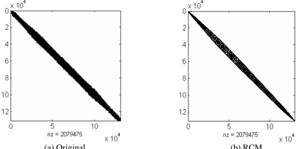
(a) Original (b) RCM
Figure 1. Nonzero pattern of the coefficient matrix from Problem 1 with Original ordering and RCM reordering.
Table 1. PCOCG with IC(0) and diagonal preconditioners for Problem 1.
Preconditioner IC(0) Diagonal preconditioner ordering NO RCM NO RCM
Its 5000 2997 755 760
By comparing Table 1 with Table 2, it is obvious that our MIC (p, τ) preconditioner is much more efficient than IC(0) and diagonal preconditioners. Observed from Tables 2 and 3, the number of iterations and total computation time of the two kinds of iterative methods of PCOCG and PCG are almost the same in all cases with the same parameters in MIC(p, τ).
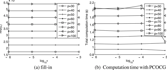
From Tables 2–4 and Fig. 1, it is noticed that the effect of dropping tolerance τ in such a wide range for Problem 1 is not prominent. Observed from Fig. 1, there is a jump of computation time with parameters p= 30andτ = 10−3. From a general view, it is a specific
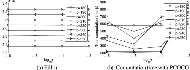
case. However, from Tables 5-7 and Fig. 2 of the test of Problem 2, it is possible for us to draw the conclusion that the effect of dropping toleranceτ is obvious in the solution of larger scale problems. And the reasonable range forτ should arrange from 10−4 to 10−6. In addition, the parameter τ has minor effect on memory requirement of our MIC preconditioner.
What affects remarkably is the parameter p which also decides both fill-ins and efficiency of MIC preconditioner. The larger p is,
(a) Original (b) RCM
Table 2. PCOCG with RCM reordering and Algorithm 6 for Problem 1.
τ p nnz(L) sp-r its P-t I-t T-t
10−3
30 171563 2.19 143 0.39 0.77 1.16 40 224771 2.88 54 0.57 0.35 0.92 50 277754 3.57 47 0.77 0.36 1.13 60 330495 4.26 39 0.97 0.33 1.30 70 382817 4.93 31 1.16 0.29 1.45 80 434926 5.61 28 1.38 0.29 1.67 90 486670 6.28 25 1.57 0.30 1.87 100 538009 6.95 23 1.78 0.27 2.05
10−4
30 171563 2.19 323 0.38 1.74 2.12 40 224774 2.88 57 0.58 0.37 0.95 50 277756 3.57 42 0.76 0.32 1.08 60 330467 4.26 38 0.96 0.32 1.28 70 382843 4.94 30 1.18 0.27 1.45 80 434934 5.61 27 1.38 0.27 1.65 90 486670 6.28 25 1.58 0.27 1.85 100 538017 6.95 22 1.77 0.26 2.03
10−5
30 171563 2.19 304 0.38 1.63 2.01 40 224774 2.88 56 0.57 0.36 0.93 50 277756 3.57 41 0.78 0.30 1.08 60 330467 4.26 38 0.98 0.32 1.30 70 382821 4.93 29 1.16 0.27 1.43 80 434934 5.61 27 1.37 0.27 1.64 90 486658 6.28 24 1.59 0.26 1.85 100 538017 6.95 22 1.78 0.27 2.05
10−6
Table 3. PCG with RCM reordering and Algorithm 6 for Problem 1.
τ p nnz(L) sp-r its P-t I-t T-t
10−3
30 171563 2.19 143 0.39 0.76 1.15 40 224771 2.88 54 0.57 0.34 0.91 50 277754 3.57 47 0.77 0.34 1.11 60 330495 4.26 39 0.96 0.32 1.28 70 382817 4.93 31 1.17 0.28 1.45 80 434926 5.61 28 1.38 0.28 1.66 90 486670 6.28 25 1.58 0.27 1.85 100 538009 6.95 23 1.77 0.26 2.03
10−4
30 171563 2.19 323 0.39 1.73 2.12 40 224774 2.88 57 0.57 0.37 0.94 50 277756 3.57 42 0.78 0.31 1.09 60 330467 4.26 38 0.98 0.32 1.30 70 382843 4.94 30 1.17 0.27 1.44 80 434934 5.61 27 1.37 0.27 1.64 90 486670 6.28 25 1.58 0.27 1.85 100 538017 6.95 22 1.78 0.26 2.04
10−5
30 171563 2.19 304 0.39 1.63 2.02 40 224774 2.88 56 0.58 0.36 0.94 50 277756 3.57 41 0.77 0.31 1.08 60 330467 4.26 38 0.97 0.31 1.28 70 382821 4.93 29 1.16 0.27 1.43 80 434934 5.61 27 1.36 0.27 1.63 90 486658 6.28 24 1.57 0.27 1.84 100 538017 6.95 22 1.78 0.27 2.05
10−6
Table 4. PCOCG with RCM reordering and Algorithm 6(τ = 0) for Problem 1.
p nnz(L) sp-r its P-t I-t T-t 30 171563 2.19 310 0.39 1.67 2.06 40 224774 2.88 57 0.57 0.38 0.95 50 277756 3.57 44 0.77 0.33 1.10 60 330467 4.26 38 0.97 0.32 1.29 70 382821 4.93 29 1.18 0.27 1.45 80 434934 5.61 26 1.37 0.28 1.65 90 486658 6.28 24 1.58 0.27 1.85 100 538017 6.95 22 1.78 0.27 2.05
the less the iteration number becomes while the more the fill-ins are required. However, the total computation time is not necessarily decreasing with the growth of p, which implies that it is crucial to select an appropriate parameter p. Generally, parameter p can be evaluated by setting the number of nonzero entries of incomplete Cholesky preconditioners, i.e., p = nnzn(L) where L is the incomplete Cholesky preconditioner and n is the dimension of coefficient matrix
A. However, the number of nonzero entries of incomplete Cholesky preconditioners L is determined by the coefficient matrix A of linear system. For small-scale linear system such as Problem 1, proper set of the number of nonzero entries ofL is about 2 times (or more) of that
6 5 4 3
1.5 2 2.5 3 3.5 4 4.5 5 5.5x 10
5
log10τ
nnz(L) p=30 p=40 p=50 p=60 p=70 p=80 p=90 p=100 (a) fill-in
6 5 4 3
0.8 1 1.2 1.4 1.6 1.8 2 2.2
log10τ
Total computation time (
s ) p=30 p=40 p=50 p=60 p=70 p=80 p=90 p=100
(b) Computation time with PCOCG
- - -
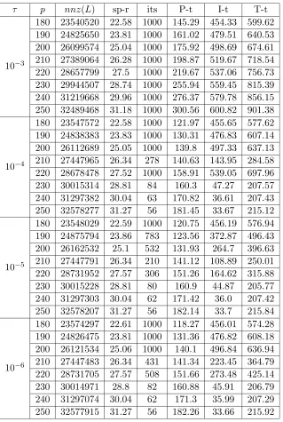
Table 5. PCOCG with RCM reordering and Algorithm 6 for Problem 2.
τ p nnz(L) sp-r its P-t I-t T-t
10−3
180 23540520 22.58 1000 148.09 454.47 602.56 190 24825650 23.81 1000 159.85 476.29 636.14 200 26099574 25.04 1000 174.97 496.12 671.09 210 27389064 26.28 1000 198.96 517.83 716.79 220 28657799 27.5 1000 219.74 537.71 757.45 230 29944507 28.74 1000 256.23 560.05 816.28 240 31219668 29.96 1000 276.74 579.14 855.88 250 32489468 31.18 1000 290.12 601.16 891.28
10−4
180 23547572 22.58 1000 121.8 455.21 577.01 190 24838383 23.83 1000 130.8 476.97 607.77 200 26112689 25.05 1000 139.76 497.00 636.76 210 27447965 26.34 278 140.69 143.99 284.68 220 28678478 27.52 1000 158.86 539.23 698.09 230 30015314 28.81 84 160.26 47.07 207.33 240 31297382 30.04 63 171.29 36.74 208.03 250 32578277 31.27 56 181.64 33.65 215.29
10−5
180 23548029 22.59 1000 120.82 455.7 576.52 190 24875794 23.86 783 122.89 372.6 495.49 200 26162532 25.1 532 131.71 264.42 396.13 210 27447791 26.34 210 141.15 108.78 249.93 220 28731952 27.57 306 151.61 164.79 316.40 230 30015228 28.81 80 160.69 44.81 205.50 240 31297303 30.04 62 171.54 36.0 207.54 250 32578207 31.27 56 182.7 33.72 216.42
10−6
Table 6. PCG with RCM reordering and Algorithm 6 for Problem 2.
τ p nnz(L) sp-r its P-t I-t T-t
10−3
180 23540520 22.58 1000 145.29 454.33 599.62 190 24825650 23.81 1000 161.02 479.51 640.53 200 26099574 25.04 1000 175.92 498.69 674.61 210 27389064 26.28 1000 198.87 519.67 718.54 220 28657799 27.5 1000 219.67 537.06 756.73 230 29944507 28.74 1000 255.94 559.45 815.39 240 31219668 29.96 1000 276.37 579.78 856.15 250 32489468 31.18 1000 300.56 600.82 901.38
10−4
180 23547572 22.58 1000 121.97 455.65 577.62 190 24838383 23.83 1000 130.31 476.83 607.14 200 26112689 25.05 1000 139.8 497.33 637.13 210 27447965 26.34 278 140.63 143.95 284.58 220 28678478 27.52 1000 158.91 539.05 697.96 230 30015314 28.81 84 160.3 47.27 207.57 240 31297382 30.04 63 170.82 36.61 207.43 250 32578277 31.27 56 181.45 33.67 215.12
10−5
180 23548029 22.59 1000 120.75 456.19 576.94 190 24875794 23.86 783 123.56 372.87 496.43 200 26162532 25.1 532 131.93 264.7 396.63 210 27447791 26.34 210 141.12 108.89 250.01 220 28731952 27.57 306 151.26 164.62 315.88 230 30015228 28.81 80 160.9 44.87 205.77 240 31297303 30.04 62 171.42 36.0 207.42 250 32578207 31.27 56 182.14 33.7 215.84
10−6
Table 7. PCOCG with RCM reordering and Algorithm 6(τ=0) for Problem 2.
p nnz(L) sp-r its P-t I-t T-t 180 23588711 22.62 1000 114.830 457.230 572.06 190 24875808 23.86 1000 123.070 476.120 599.19 200 26161974 25.09 428 131.940 214.42 346.36 210 27447316 26.33 1000 144.280 518.570 662.85 220 28731527 27.57 212 151.670 114.240 265.91 230 30014648 28.80 81 160.750 45.350 206.10 240 31296689 30.03 63 172.080 36.700 208.78 250 32577809 31.26 56 184.360 33.680 218.04
of A. For middle-scale linear system such as Problem 2, the select of the number of nonzero entries ofLcould be 5 (or more) times of that of A.
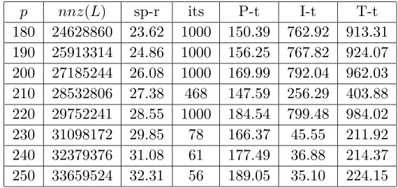
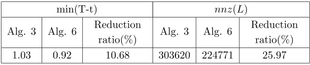
In order to compare the performance of Algorithm 4 (MIC(p,τ) with that of Algorithm 3, numerical experiments with Algorithm 3 are also performed. Note that parameter p in Algorithms 3 and 4 has different meanings. Observed from Tables 8 and 9, Algorithm 3 needs more memory than Algorithm 4 under the requirement of the same total computation time. Take Problem 2 for example. The minimum computation time with Algorithm 3 is 211.92(s) and the fill-ins ofL is 31098172. Nevertheless, using Algorithm 4, it consumes
6 5 4 3
2.2 2.4 2.6 2.8 3 3.2 3.4x 10
7 log 10τ nnz(L) p=180 p=190 p=200 p=210 p=220 p=230 p=240 p=250 (a) Fill-in
6 5 4 3
200 300 400 500 600 700 800 900 log 10τ
Total computation time (
s
) p=180
p=190 p=200 p=210 p=220 p=230 p=240 p=250
(b) Computation time with PCOCG
- - -
Table 8. PCOCG with RCM reordering and Algorithm 3 for Problem 1.
p nnz(L) sp-r its P-t I-t T-t 10 143492 1.83 1000 0.13 4.66 4.79 15 170548 2.18 985 0.19 5.12 5.31 20 197289 2.53 355 0.25 2.04 2.29 25 223975 2.87 213 0.33 1.34 1.67 30 250578 3.22 146 0.42 0.97 1.39 40 303620 3.91 55 0.61 0.42 1.03 50 356219 4.59 43 0.81 0.37 1.18 60 408503 5.27 38 1.00 0.36 1.36 70 460516 5.94 30 1.20 0.32 1.52 80 512103 6.61 26 1.40 0.30 1.70 90 563380 7.28 24 1.61 0.29 1.90 100 614174 7.94 23 1.82 0.31 2.13
Table 9. PCOCG with RCM reordering and Algorithm 3 for Problem 2.
p nnz(L) sp-r its P-t I-t T-t 180 24628860 23.62 1000 150.39 762.92 913.31 190 25913314 24.86 1000 156.25 767.82 924.07 200 27185244 26.08 1000 169.99 792.04 962.03 210 28532806 27.38 468 147.59 256.29 403.88 220 29752241 28.55 1000 184.54 799.48 984.02 230 31098172 29.85 78 166.37 45.55 211.92 240 32379376 31.08 61 177.49 36.88 214.37 250 33659524 32.31 56 189.05 35.10 224.15
205.5(s) with parameters p = 230and τ = 10−5 and the fill-ins of L
Table 10. Comparison results with respect to the minimum of total computation time and the corresponding memory between Algorithms 3 and 6 for Problem 1.
min(T-t) nnz(L)
Alg. 3 Alg. 6 Reduction
ratio(%) Alg. 3 Alg. 6
Reduction ratio(%) 1.03 0.92 10.68 303620 224771 25.97
5. CONCLUSIONS
A column-oriented modified incomplete Cholesky factorization MIC (p, τ) with two controlling parameters for solution of systems of linear equations with sparse complex symmetric coefficient matrices resulted from finite-element analysis of the electromagnetic scattering problem (1) is presented in this paper. Proper choices of the controlling parameters in Algorithm 6 can evidently reduce the total computation time and memory requirements compared with Algorithm 3. It is worthwhile to emphasize that the involved parameter p, which prescribes the maximal fill-ins in each row of preconditioners, makes Algorithm 6 evidently superior to Algorithm 3 in the number of fill-ins, and helps to reduce total computation time of Algorithm 6. As shown in the numerical experiments, RCM ordering is obviously superior to AMD ordering. Moreover, RCM ordering is significant to our modified incomplete Cholesky factorization. Numerical experiments show that further developments of more proper incomplete factorization algorithms and reordering schemes for electromagnetic scattering problems are deserved to be taken into consideration in the future. ACKNOWLEDGMENT
REFERENCES
1. Jin, J. M.,The Finite Element Method in Electromagnetics, Wiley, New York, 1993.
2. Volakis, J. L., A. Chatterjee, and L. C. Kempel, Finite Element Method for Electromagnetics: Antennas, Microwave Circuits and Scattering Applications, IEEE Press, New York, 1998.
3. Ahmed, S. and Q. A. Naqvi, “Electromagnetic scattering of two or more incident plane waves by a perfect, electromagnetic conductor cylinder coated with a metamaterial,” Progress In Electromagnetics Research B, Vol. 10, 75–90, 2008.
4. Fan, Z. H., D. Z. Ding, and R. S. Chen, “The efficient analysis of electromagnetic scattering from composite structures using hybrid CFIE-IEFIE,”Progress In Electromagnetics Research B, Vol. 10, 131–143, 2008.
5. Botha, M. M. and D. B. Davidson, “Rigorous auxiliary variable-based implementation of a second-order ABC for the vector FEM,” IEEE Trans. Antennas Propagat., Vol. 54, 3499–3504, 2006.
6. Harrington, R. F., Field Computation by Moment Method, 2nd edition, IEEE Press, New York, 1993.
7. Choi, S. H., D. W. Seo, and N. H. Myung, “Scattering analysis of open-ended cavity with inner object,” J. of Electromagn. Waves and Appl., Vol. 21, No. 12, 1689–1702, 2007.
8. Ruppin, R., “Scattering of electromagnetic radiation by a perfect electromagnetic conductor sphere,”J. of Electromagn. Waves and Appl., Vol. 20, No. 12, 1569–1576, 2006.
9. Ho, M., “Scattering of electromagnetic waves from, vibrating per-fect surfaces: Simulation using relativistic boundary conditions,” J. of Electromagn. Waves and Appl., Vol. 20, No. 4, 425–433, 2006. 10. Lin, C.-J. and J. J. More, “Incomplete cholesky factorizations with
limited memory,”SIAM J. Sci. Comput., Vol. 21, 24–45, 1999. 11. Fang, H.-R. and P. O. Dianne, “Leary, modified Cholesky
algorithms: A catalog with new approaches,” Mathematical Programming, July 2007.
12. Margenov, S. and P. Popov, “MIC(0) DD preconditioning of FEM elasticity problem on non-structured meshes,” Proceedings of ALGORITMY 2000 Conference on Scientific Computing, 245– 253, 2000.
14. Freund, R. and N. Nachtigal, “A quasi-minimal residual method for non-Hermitian linear systems,” Numer. Math., Vol. 60, 315– 339, 1991.
15. Van der Vorst, H. A. and J. B. M. Melissen, “A Petrov-Galerkin type method for solvingAx=b, whereA is symmetric complex,” IEEE Trans. Mag., Vol. 26, No. 2, 706–708, 1990.
16. Barrett, R., M. Berry, T. F. Chan, J. Demmel, J. Donato, J. Don-garra, V. Eijkhout, R. Pozo, C. Romine, and H. van der Vorst, Templates for the Solution of Linear Systems: Building Blocks for Iterative Methods, 2nd edition, SIAM, Philadelphia, PA, 1994. 17. Saad, Y., Iterative Methods for Sparse Linear Systems, 2nd
edition, SIAM, Philadelphia, PA, 2003.
18. Saad, Y., “Sparskit: A basic tool kit for sparse matrix computations,” Report RIACS-90-20, Research Institute for Advanced Computer Science, NASA Ames Research Center, Moffett Field, CA, 1990.
19. Benzi, M., “Preconditioning techniques for large linear systems: A survey,”J. Comp. Physics, Vol. 182, 418–477, 2002.
20. Meijerink, J. A. and H. A. van der Vorst, “An iterative solution method for linear equations systems of which the coefficient matrix is a symmetric M-matrix,”Math. Comp., Vol. 31, 148–162, 1977. 21. Lee, I., P. Raghavan, and E. G. Ng, “Effective preconditioning through ordering interleaved with incomplete factorization,”Siam J. Matrix Anal. Appl., Vol. 27, 1069–1088, 2006.
22. Ng, E. G. and P. Raghavan, “Performance of greedy ordering heuristics for sparse Cholesky factorization,”Siam J. Matrix Anal. Appl., Vol. 20, No. 2, 902–914, 1999.
23. Benzi, M., D. B. Szyld, and A. van Duin, “Orderings for incomplete factorization preconditioning of nonsymmetric problems,” SIAM J. Sci. Comput., Vol. 20, 1652–1670, 1999. 24. Benzi, M., W. Joubert, and G. Mateescu, “Numerical experiments
with parallel orderings for ILU preconditioners,” Electronic Transactions on Numerical Analysis, Vol. 8, 88–114, 1999. 25. Chan, T. C. and H. A. van der Vorst, “Approximate
and incomplete factorizations,” Preprint 871, Department of Mathematics, University of Utrecht, The Netherlands, 1994. 26. Zhang, Y., T.-Z. Huang, and X.-P. Liu, “Modified iterative