Future changes of hydroclimatic extremes in western North America using a large ensemble: The role of internal variability

(1)

Scholarship@Western

Electronic Thesis and Dissertation Repository

4-16-2019 1:45 PM

Future changes of hydroclimatic extremes in western North

America using a large ensemble: The role of internal variability

Mohammad Hasan Mahmoudi

The University of Western Ontario

Supervisor Najafi, Reza

The University of Western Ontario

Graduate Program in Civil and Environmental Engineering

A thesis submitted in partial fulfillment of the requirements for the degree in Master of Science © Mohammad Hasan Mahmoudi 2019

Follow this and additional works at: https://ir.lib.uwo.ca/etd

Part of the Environmental Engineering Commons, Environmental Indicators and Impact Assessment Commons, Hydraulic Engineering Commons, Other Civil and Environmental Engineering Commons, and the Water Resource Management Commons

Recommended Citation Recommended Citation

Mahmoudi, Mohammad Hasan, "Future changes of hydroclimatic extremes in western North America using a large ensemble: The role of internal variability" (2019). Electronic Thesis and Dissertation Repository. 6151.

https://ir.lib.uwo.ca/etd/6151

This Dissertation/Thesis is brought to you for free and open access by Scholarship@Western. It has been accepted for inclusion in Electronic Thesis and Dissertation Repository by an authorized administrator of

(2)

I

Increases in the intensity and frequency of extreme events in Western North America (WNA)

can cause significant socioeconomic problems and threaten existing infrastructure. In this study

we analyze the impacts of climate change on hydroclimatic extremes and assess the role of

internal variability over WNA, which collectively drain an area of about 1 million km2. We

used gridded observations and downscaled precipitation, maximum and minimum temperature

from seven General Circulation Models (GCMs) that participated in the Coupled Model

Intercomparison Project Phase 5 (CMIP5) and a large ensemble of CanESM2 model

simulations (CanESM2-LE; 50 members) for this analysis. Spatial and temporal changes of

eight climate extreme indices are assessed over the historical (1981-2010) and future

(2060-2089) time periods. In addition, changes in extreme events with high return periods are

analyzed based on the extreme value theory. To better understand the effects of internal climate

variability on the hydroclimatology of WNA we assess the relations between 14 Low

Frequency Variability Modes (LFVMs), with three different time lags, and the regional

temperature and precipitation. The correlation between each LFVM and the principle

component of temperature and precipitation over the spatial domain is computed using

Maximum Covariance Analysis (MCA). Robustness of the results is further evaluated using

composite analysis. Results show that the intensity and frequency of extreme precipitation and

temperature are projected to increase over WNA. The uncertainties due to internal variability

(represented by CanESM2-LE) are significant and comparable to those arising from GCM

structures. El Nino Southern Oscillation, Trans-Polar Index (TPI), Southern Annular Mode

(SAM), Eastern Pacific (EP) and West Pacific (WP) are found to be dominant LFVMs that can

(3)

II

Hydroclimatic extremes, climate change, internal variability, precipitation, temperature,

runoff, western North America, Low frequency variability mode, CLIMDEX, composite

(4)

III

First and foremost, I would like to thank the brain for its never-ending grace, mercy and

provision during challenging times of my life. Although, I need to apologize to it for not being

able to use all of it.

I would like to thank my thesis advisor Dr. Mohammad Reza Najafi, my patient supervisor

whose office’s door was always open whenever I ran into a problem or had a question about

my research or writing.

I would like to thank my research group and the experts who provided passionate support

throughout my study including Dr. Alireza Massah, Mohammad Sadeq Abbasian and Harry

Singh. I also thank Markus Schnorbus and Arelia Werner from Pacific Climate Impacts

Consortium who provided downscaled climate model simulations and gridded observations

over western North America; and Dr. George Josh, BC Hydro, for sharing the calibrated

hydrological model.

Finally, I must express my very profound gratitude to my parents (Maman Pouri and Baba

Reza), to my girlfriend and future wife Brianna Ananthan and my best friend Dr. Erfun

Asadipour for providing me with unfailing support and continuous encouragement throughout

my years of study and through the process of researching and writing this thesis. This

(5)

IV

Abstract ... I

Acknowledgement ... III

Table of Contents ... IV

List of tables ... VII

List of Figures ... VIII

Acronyms ... XV

Chapter 1 ... 1

1. Introduction ... 1

1.1. Hydroclimatic extreme events ... 1

1.2. Changes in extreme events ... 2

1.2.1 Impacts of climate change on extreme events ... 3

1.2.2 Internal variability ... 6

1.3. Research Objectives ... 9

1.4. Research questions ... 10

1.5. Thesis organization ... 10

Chapter 2 ... 11

2. Literature review ... 11

2.1. Assessment of Climate Change Impacts on Hydroclimatic Extremes ... 11

2.2. Impacts of LFVMs ... 15

(6)

V

3.1. Study area ... 18

3.2. Data ... 22

3.2.1. Daily Gridded Observation ... 23

3.2.2. General Circulation Models ... 23

3.3. Methods ... 26

3.5.1. Climate extreme indices ... 27

3.5.2. Generalized Extreme Value Distribution ... 30

3.5.3. Composite Analysis ... 32

3.5.4. Maximum Covariance Analysis ... 34

Chapter 4 ... 37

4. Results and discussion ... 37

4.1. Temporal changes of the annual maximum precipitation and temperature ... 37

4.2. Spatial changes in indices of extreme precipitation and temperature for WNA ... 43

4.3 Temporal changes of extreme indices ... 49

4.4. Spatial distributions of extreme Pr&T with 50- and 100-year return levels ... 55

4.5. Impacts of low frequency variability modes on WNA’s hydroclimatic variables ... 59

4.6. Streamflow ... 72

Chapter 5 ... 78

5. Conclusion ... 78

(7)

VI

(8)

VII

Table 1. LFVMs and their indices ... 8

Table 2.GCMs used in this study ... 25

Table 3.Climate extreme indices (CLIMDEX) that are analyzed in this study ... 28

Table 4.The changes of AM from historical to future period over WNA (FRB, PRB, CRB,

CaRB) ... 38

Table 5. Same as table 4 but in percentage ... 38

Table 6. P-factors of CanESM2_LE and SR_GCMs for four key river basins over WNA (FRB,

PRB, CRB, CaRB) ... 43

Table 7. R-factors of CanESM2_LE and SR_GCMs for four key river basins over WNA (FRB,

PRB, CRB, CaRB) ... 43

Table 8. P-factor and R-factor of CanESM2_LE and SR_GCMs for TNN, TXX, CDD and

GSL ... 53

Table 9. P-factor and R-factor of CanESM2_LE and SR_GCMs for R10, R95PTOT, RX5day

and SDII ... 55

Table 10. 5 lowest and highest LFVM years ... 63

(9)

VIII

Figure 1.Global mean surface temperature (Hansen et al., 2010)... 4

Figure 2. Four key river basins in WNA (light green: FRB, beige: PRB, purple: CRB, blue: CaRB) ... 21

Figure 3. Kootenay River Basin ... 22

Figure 4. Methodology flowchart ... 27

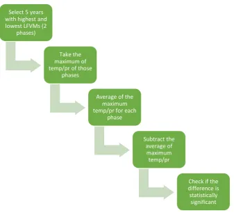
Figure 5. Composite Analysis flowchart... 33

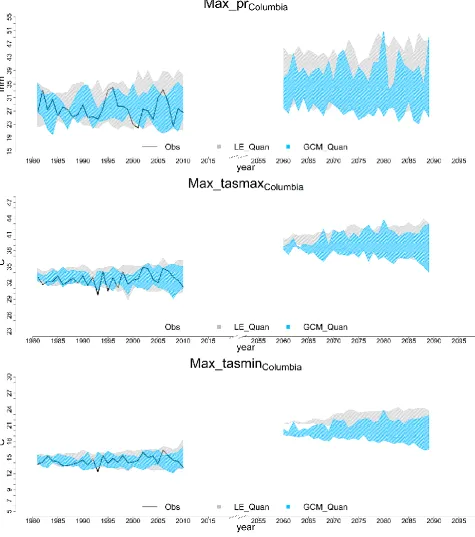
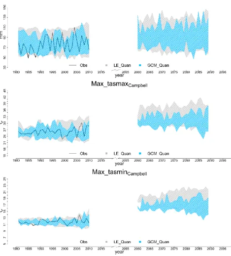
Figure 6. Changes in the AM precipitation, tasmax and tasmin over FRB. The black solid line represents the observations; blue and red shades show the 95th quantiles of seven GCMs and 50 CanESM2-LE runs, respectively, over historical (1981-2010) and future (2060-2089) periods. ... 40

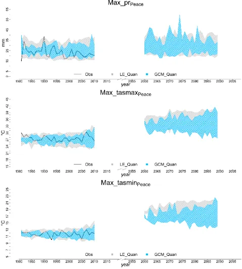
Figure 7. Changes in the AM precipitation, tasmax and tasmin over PRB. The black solid line represents the observations; blue and red shades show the 95th quantiles of seven GCMs and 50 CanESM2-LE runs, respectively, over historical (1981-2010) and future (2060-2089) periods. ... 40

Figure 8. Changes in the AM precipitation, tasmax and tasmin over CRB. The black solid line represents the observations; blue and red shades show the 95th quantiles of seven GCMs and 50 CanESM2-LE runs, respectively, over historical (1981-2010) and future (2060-2089) periods. ... 41

(10)

IX

CanESM2_LE and SR_GCM simulations over the historical (1981-2010) (first rows) and

future (2060-2089) (second rows) periods over WNA ... 45

Figure 11. Spatial average Changes of CDD and GSL based on gridded observations,

Figure 12. Monthly variation of RX5day, TXX and TNN based on gridded observations (black

dashed line), CanESM2_LE and GCM simulations for historical (1981-2010) (green and blue

dashed line associated with CanESM2_LE and SR_GCMs, respectively) and future

(2060-2089) (red and brown dashed line associated with CanESM2_LE and SR_GCMs, respectively)

periods ... 50

Figure 13. Historical (1981-2010) and projected (2060-2089) changes of TNN, TXX, CDD

and GSL based on gridded observation (solid black line), CanESM2_LE (left side) and

SR_GCM (right side) simulations. Red and blue dashed lines are 95th_{quantile of simulations}

(CanESM2_LE on the left and SR_GCMs on the right side) for historical and projection period,

respectively. Solid green line is the temporal average of CanESM2_LE/SR_GCM simulations.

The solid red and blue lines are the mean of the historical and projection period, respectively.

... 52

Figure 14. Historical (1981-2010) and projected (2060-2089) changes of R10, R95PTOT,

RX5day and SDII based on gridded observation (solid black line), CanESM2_LE (left side)

and SR_GCM (right side) simulations. Red and blue dashed lines are 95th quantile of

simulations (CanESM2_LE on the left and SR_GCMs on the right side) for historical and

projection period, respectively. Solid green line is the temporal average of

CanESM2_LE/SR_GCM simulations. The solid red and blue lines are the mean of the

(11)

X

and on future period (2060-2089) (second row) over WNA using gridded observation (left

column), CanESM2_LE (middle column) and SR_GCM (right column) simulations. ... 56

Figure 16. Tasmax 50-year return level based on historical period (1981-2010) (first row) and

on future period (2060-2089) (second row) over WNA using gridded observation (left column),

CanESM2_LE (middle column) and SR_GCM (right column) simulations. ... 57

Figure 17. Tasmin 50-year return level based on historical period (1981-2010) (first row) and

on future period (2060-2089) (second row) over WNA using gridded observation (left column),

CanESM2_LE (middle column) and SR_GCM (right column) simulations. ... 57

Figure 18. Correlation between LFVMs signals using three lags (no lag, one month lag, two

months lag) and expansion coefficient of average temperature... 60

Figure 19. Correlation between LFVMs using three lags (no lag, one month lag, two months

lag) and expansion coefficient of average precipitation ... 61

Figure 20. Correlation between LFVMs using three lags (no lag, one month lag, two months

lag) and expansion coefficient of maximum precipitation ... 62

Figure 21. Differences in the extended winter hydroclimatic variables (Precipitation: first row,

maximum temperature: second row, minimum temperature: third row) averaged from 5 years

associated with highest and lowest value of EA with three different lags (no lag: first column,

one month lag: second column, two months lag: third column). Shadowed areas are those grids

whose differences are statistically significant... 66

associated with highest and lowest value of NAO with three different lags (no lag: first column,

(12)

XI

associated with highest and lowest value of Nino3.4 with three different lags (no lag: first

column, one month lag: second column, two months lag: third column). Shadowed areas are

those grids whose differences are statistically significant. ... 68

associated with highest and lowest value of NTA with three different lags (no lag: first column,

associated with highest and lowest value of WP with three different lags (no lag: first column,

Figure 26.Temporal streamflow based on gridded observation (first row), CanESM2_LE

(second row) and GCMs (third row) ... 73

Figure 27. 95th quantile of historical and future simulated streamflow based on GCMs (blue

shadow) and observed streamflow based on gridded observation (solid black line) ... 74

Figure 28. 95th quantile of historical and future simulated streamflow based on CanESM2_LE

(blue shadow) and observed streamflow based on gridded observation (solid black line) ... 75

Figure 29. Maximum daily streamflow over the KRB based on observed gridded observation

(black line), CanESM2_LE (red line) and GCMs (green line) over historical (top) and future

(13)

XII

Appendix 2. Spatial average Changes of RX5day and SDII based on gridded observations,

Appendix 3. Precipitation 100-year return level based on historical period (1981-2010) (first

row) and on future period (2060-2089) (second row) over WNA using gridded observation (left

Appendix 4. Tasmax 100-year return level based on historical period (1981-2010) (first row)

Appendix 5. Tasmin 100-year return level based on historical period (1981-2010) (first row)

Appendix 6. Differences in the extended winter hydroclimatic variables (Precipitation: first

row, maximum temperature: second row, minimum temperature: third row) averaged from 5

years associated with highest and lowest value of AO with three different lags (no lag: first

years associated with highest and lowest value of DMI with three different lags (no lag: first

(14)

XIII

years associated with highest and lowest value of EP with three different lags (no lag: first

years associated with highest and lowest value of ONI with three different lags (no lag: first

years associated with highest and lowest value of PDO with three different lags (no lag: first

years associated with highest and lowest value of PNA with three different lags (no lag: first

years associated with highest and lowest value of SAM with three different lags (no lag: first

(15)

XIV

years associated with highest and lowest value of SOI with three different lags (no lag: first

years associated with highest and lowest value of TPI with three different lags (no lag: first

(16)

XV

*.nc = NetCDF ... 23

ACCESS1-0 =ARC Centre of Excellence for Climate System Science... 25

ACCESS1-3 =ARC Centre of Excellence for Climate System Science... 25

AO = Arctic Oscillation ... 8

BCCA = Bias Correction Constructed Analogues ... 25

BCCAQ = Bias Correction/Constructed Analogues with Quantile mapping reordering approach ... 24

BCCI = Bias Corrected Climate Imprint ... 25

CanESM2 =Canadian Centre for Climate Modelling and Analysis ... 25

CanESM2-LE =CanESM2- Large Ensemble ... 26

CaRB = Campbell River Basin ... 20

CCA = Canonical Correlation Analysis ... 35

CCSM4 =University Corporation for Atmospheric Research (UCAR) ... 25

CDD = maximum number of consecutive dry days... 5

CLIMDEX = Climate extreme indices ... 4

CMIP3 = Coupled Model Intercomparison Project Phase 3 ... 11

CMIP5 = Coupled Model Intercomparison Project Phase 5 ... 11

CNRM-CM5 =Centre National de Recherches Meteorologiques / Centre Europeen de Recherche et Formation Avancees en Calcul Scientifique ... 25

CRB = Columbia River Basin ... 16

DMI =Dipole Mode Index ... 8

EA =East Atlantic ... 8

(17)

XVI

EP =Eastern Pacific ... 8

ETCCDI = Expert Team on Climate Change Detection and Indices ... 11

EVT = Extreme Value Theory ... 5

FRB = Fraser River Basin ... 18

GEV = Generalized Extreme Value ... 14

GP = generalized Pareto ... 30

GSL = Growing Season Length ... 5

HadGEM2-ES =Met Office Hadley Centre ESM ... 25

HIV = Human Immunodeficiency Viruses ... 1

IPCC = Intergovernmental Panel on Climate Change ... 3

MCA = Maximum Covariance Analysis ... 9

MCA1 = MCA mode 1 ... 59

MPI-ESM-LR =Max Planck Institute for Meteorology (MPI-M) ... 25

NAO =North Atlantic Oscillation ... 8

NP = North Pacific ... 17

NTA =North Tropical Atlantic ... 8

PC = Principal Component ... 16

PDF = Probability Density Function ... 31

PDO =Pacific Decadal Oscillation ... 8

PDSI = Palmer Drought Severity Index ... 16

PNA =Pacific/North American Pattern ... 8

R10 = number of days with precipitation greater than 10 mm ... 5

(18)

XVII

RCP = Representative Concentration Pathway... 3

RX5day = monthly maximum consecutive 5-day precipitation ... 5

SAM = Southern Annular Mode ... 8

SCF = Square Covariance Fraction ... 36

SDII = simple precipitation intensity index ... 5

SOI =Southern Oscillation Index ... 8

SST = Sea Surface Temperature ... 16

SVD = Singular Value Decomposition ... 16

tasmax = maximum daily temperature ... 32

tasmin = minimum daily temperature ... 32

TNn = minimum Temperature ... 5

TPI =Trans Polar Index ... 8

TXx = maximum temperature ... 5

UPRB = Upper Peace River Basin... 19

(19)

1

Chapter 1

1. Introduction

This section discusses hydroclimatic extreme events (including precipitation, temperature and

runoff), their driving mechanisms, examples of historical events, and the role of climate change

and internal variability followed by the thesis outline in the end.

1.1. Hydroclimatic extreme events

Definition of extreme events varies between different disciplines. Politicians and journalists

define them as any event with an important consequence. According to this definition, a heavy

rainfall that cause no flooding is not considered an extreme event. Pandemics such as HIV or

flu are extreme societal events. Other examples include large benefit/loss in market turbulence,

embezzlement in politics, earthquake and landslide in geoscience, flood and drought in natural

science. Hydrologists define extreme events as deviations from the usual trend of the observed

or simulated variable (such as precipitation, temperature, runoff), or as unusual/unexplainable

events regardless of their impacts (Albeverio, Jentsch and Kantz, 2006). In general, the tails of

a probability distribution of a variable are considered as extremes.

Extreme events, such as floods and droughts, commonly occur in North America (NA) as well

as other regions around the world resulting in significant socioeconomic consequences.

Examples include flooding in central Arizona on July 24th in 1990, which was initiated by

heavy rainfall and locally strong winds. Texas faced severe drought conditions starting from

October 2010 with an average precipitation amount of 14.8 inches recorded in 2011, as the

(20)

2

predicted based on above-average snow survey records in February. Temperature rise

contributed to snowmelt in May 2018 and resulted in massive flooding in British Columbia as

well. It caused thousands of residents to be displaced in Grand Forks, Osoyoos with some on

alert in Chilliwack.

Increases in the severity and frequency of extreme events, due to natural or human-induced

causes, can result in severe damages and losses in the future. Understanding historical changes

of the characteristics of extremes and the driving mechanisms is essential for their accurate

future predictions.

1.2. Changes in extreme events

According to the Clausius-Clapeyron relationship increases in the atmospheric temperature

would raise its moisture holding capacity resulting in more severe and more frequent extreme

events. Therefore, in a changing climate more intense flooding, caused by heavier rainfall

among others, are expected to occur in many regions around the world particularly the ones

that are categorized as wet areas. Temperature increases would also increase the

evapotranspiration rates and reduce the average rainfall rates particularly in dry areas resulting

in severe drought conditions. Therefore, societies and infrastructure are more vulnerable to

hydroclimatic extreme events under climate change. In addition, internal climate variability,

due to the chaotic nature of the atmospheric and oceanic processes play a significant role in

(21)

3

1.2.1 Impacts of climate change on extreme events

Climate is an average state of weather prevailing in an area over a long period of time. The

global climate has always been oscillating, however observational data shows that the average

global temperature has been increasing over the past decades particularly since 1980s. There is

strong evidence that these observed changes are associated with anthropogenic greenhouse

effects caused by human-induced emissions via industrialization (Najafi et al., 2015).

Greenhouse gasses (GHGs), including carbon dioxide, methane, water-vapor, nitrous oxide,

among others, can trap the long-wave radiation emitted from the Earth’s surface into the

atmosphere resulting in increases in the Earth’s surface temperature. Since 19th century global

GHG concentrations have been increasing steadily (van Vuuren et al., 2011). Because of the

lack of knowledge of future GHG concentrations, the Intergovernmental Panel on Climate

Change (IPCC) has introduced four distinct GHG emission scenarios, representing possible

range of future GHG concentrations, called Representative Concentration Pathways (RCPs)

2.6, 4.5, 6.0 and 8.5 (Stocker et al., 2013). Total radiative forcing, which is a cumulative

measure of human emissions of GHG levels, is used to define different RCPs by the end of

2100.

The global average temperature has increased by 2°C over the past 35 years because of the

human influence (Northon, 2017). Although the average rate of temperature changes is not

large (compared to daily and seasonal variations), even the consequences of small temperature

changes are significantly destructive. Rising temperature can intensify the hydrological cycle

and increase the severity and frequency of extremes through increased evapotranspiration,

snow cover declines, glacial retreats, rising sea levels, warming oceans, shrinking ice sheets,

heavy rainfall, among others (Wuebbles, Fahey and Hibbard, 2017). These changes can

(22)

4

sea levels, warming oceans, shrinking ice sheets and extreme events (Wuebbles, Fahey and

Hibbard, 2017).

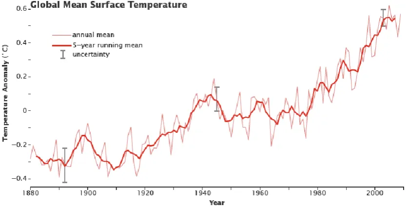
Figure 1.Global mean surface temperature (Hansen et al., 2010)

As Figure 1 shows two main characteristics of the global mean surface temperature changes

including climate signals, i.e. the long-term trends and projections of the climate system, and

noise, i.e. internal climate variability. The climate signal (or the forced response) represents the

effects of climate change or the fingerprints of anthropogenic GHG emissions in long-term

temperature trends. In this study we analyze the impacts of climate change on hydroclimate

extremes using parametric and non-parametric statistical methods.

Statistical analysis is required to analyze the impacts of climate change on extreme events and

quantify the uncertainties. In this study, we use parametric and non-parametric methods based

on Extreme Value Theory (EVT) and climate extreme indices (CLIMDEX), which are

quantitative metrics that show changes in extreme temperature and precipitation at the monthly

(23)

5

data that are defined by the Expert Team on Climate Change Detection and Indices (ETCCDI)

(Karl, Nicholls and Ghazi, 1999a; Zhang et al., 2005). In this study, CLIMDEX indices are

used to assess spatial and temporal variability of hydroclimatic extremes, quantify the

uncertainties in climate change impacts on extremes, evaluate GCMs, and characterize climate

signal and internal variability of extremes.

We selected eight CLIMDEX indices, which represent the intensity (I) and frequency (F) of

extreme Pr &T (e.g. growing length, drying days, very high precipitation etc.). These include

three temperature-based indices: Growing Season Length (GSL; F), maximum temperature

(TXx; I), minimum Temperature (TNn; I); and five precipitation indices including the number

of days with precipitation greater than 10 mm (R10; F), monthly maximum consecutive 5-day

precipitation (RX5day; I), simple precipitation intensity index (SDII; I), total amount of

precipitation exceeding the 95th percentile of the climatological distribution for wet days (i.e.

daily RR ≥ 1.0mm) (R95pTOT; F), and maximum number of consecutive dry days (i.e. RR <

1mm; F) (CDD), which is a precipitation based drought index.

Additionally, we analyzed extreme precipitation and temperature values at the tails of their

corresponding probability distributions. Extreme Value Theory (EVT) was used to analyze the

stochastic behavior of extreme values and characterize events that have relatively long return

periods (~100 years). Extreme value distributions are fitted to the observed and simulated

extremes over the historical and future periods, the corresponding parameters are inferred using

available methods such as Maximum Likelihood Estimation (MLE), and extreme events with

(24)

6

Impacts of climate change on streamflow

Increases in the intensity and frequency of hydroclimatic extremes (Touma et al., 2015; Pagán

et al., 2016) would challenge water resources management. For example, lengthening drought

durations in arid and semi-arid regions can cause difficulties in releasing the minimum

environmental flows from the reservoirs. Increases in precipitation, however, demands more

storage in reservoirs and attention for downstream water releases (Carlton and Kandathil,

2013). Therefore, any changes in hydroclimatic variables, especially precipitation, can have

significant consequences for recreational activities, dam operations, ecosystems and water

quality upstream and downstream of the reservoirs (Naz et al., 2018).

To better understanding the impact of climate change on streamflow, we use a hydrological

model (setup and calibrated by BC-Hydro) to assess the projected changes of regional

streamflow.

1.2.2 Internal variability

Internal variability originates from internal processes within the climate system and the

interactions between the atmosphere, ocean and land surface components (i.e. soil, vegetation

etc.). Characterization and prediction of internal variability (noise; Figure 1) are quite

challenging because of the complexities that exist in this natural system. However it is critical

to understand and distinguish the influence of internal climate variability and forcing signals

on hydroclimatic extremes for future policy making, and planning and design of civil

(25)

7

variability are more noticeable in precipitation compared to temperature particularly at regional

scales (Deser, Knutti, et al., 2012; Fischer, Beyerle and Knutti, 2013; Xie et al., 2015).

Low Frequency Variability Modes (LFVMs)

Large-scale atmospheric circulations can affect the regional weather patterns of many regions

around the world and last for several days, weeks, months, or years. LFVMs are large-scale

anomalies that refer to periodic patterns of pressure and circulation over a vast area. The chaotic

changes of the sea-level pressure between two regions can lead to changes in sea surface

temperature (SST) that can affect the hydroclimate of many regions around the world. Low

Frequency Variability Modes (LFVMs) are generally defined based on the anomalies of

pressure or temperature at a specific time period. There are several teleconnection patterns that

span over the Pacific and Atlantic oceans including El Niño Southern Oscillation (ENSO),

which is defined as the anomaly of spatially averaged SST over the equatorial Pacific Ocean).

Since teleconnection patterns commonly remain for a relatively long time (they might last for

weeks to several years), they are also referred to as preferred modes of low-frequency

variability.

The most common and important LFVMs affecting NA are associated with the anomalies that

occur over the Pacific and Atlantic oceans including changes in the tropical SSTs (Barnston et

al., 1991). The well-known examples of internally generated variabilities in North America

(NA) include Pacific Decadal Oscillation (PDO), ENSO, Atlantic Multidecadal Oscillation

(AMO) and North Atlantic Oscillation (NAO). ENSO is known as one of the most influential

(26)

8

analyzed the effects of 14 teleconnection signals on hydroclimatic extremes over western North

America (WNA; Table 1).

Table 1. LFVMs and their indices

Teleconnection name Abbreviation

Arctic Oscillation AO

Dipole Mode Index DMI

East Atlantic EA

Eastern Pacific EP

North Atlantic Oscillation NAO

El Niño-Southern Oscillation Nino3.4

North Tropical Atlantic NTA

El Niño-Southern Oscillation ONI

Pacific Decadal Oscillation PDO

Pacific/North American Pattern PNA

Southern Annular Mode SAM

Southern Oscillation Index SOI

Trans Polar Index TPI

West Pacific WP

Teleconnection impacts on extreme events

Considering that LFVMs can influence regional hydroclimatic variables, there are two main

questions that need to be addressed: which teleconnection signals can affect the hydroclimatic

variables at a specific region? and how much can they explain the hydroclimatic variabilities?

We used two statistical approaches to address these questions including composite analysis and

maximum covariance analysis.

Composite analysis is a straightforward, non-parametric approach to analyze basic structural

(27)

9

variability modes on regional extremes (Zhang et al., 2010). Maximum Covariance Analysis

(MCA) is a systematic approach to characterize the relationships between LFVMs and

hydroclimatic variables. MCA analyzes the patterns, between a spatio-temporally varying

hydroclimatic variable and LFVMs, which explain a maximum fraction of covariance between

them. Wilks, (2015) showed that MCA is a suitable approach to capture atmospheric and

oceanic processes. MCA analyzes the dominant modes of interaction robustly because of its

comprehensive assessment of the relationship between the space-time datasets (Frankignoul,

Chouaib and Liu, 2011).

1.3. Research Objectives

The overall objective of this research is to assess the observed and projected changes of

hydroclimatic extreme events in WNA and understand the driving mechanisms. The first

objective is to evaluate simulated changes of extreme hydroclimatic variables based on a Large

Ensemble (LE) of downscaled General Circulation Models (GCMs) using gridded observations

over western NA. The second objective is to assess future spatial and temporal changes in

extreme Pr&T under climate change. The third objective is to characterize the uncertainties in

GCM structures and model initialization and understand the roles of climate change and

internal variability in characterizing extremes. The fourth objective is to quantify the influence

of LFVMs on extremes over the study region. And the fifth objective is to assess projected

changes in runoffs in selected watersheds in western NA using the large suite of downscaled

(28)

10

1.4. Research questions

The following questions are addressed in this research:

 How do the spatial patterns of observed and GCM simulated extreme events compare

in terms of both frequency and intensity?

 How do frequency and intensity of extreme events in WNA change under climate

change?

 Are there consistencies between parametric and non-parametric analyses of extreme

events?

 What are the uncertainties of GCMs? Are they reliable for further studies over the

region?

 What is the relationship between LFVMs and hydroclimatic variables? Which

LFVMs affect hydroclimatic variables in WNA and to what extent?

 What are projected changes in streamflow over the region?

1.5. Thesis organization

Chapter 2 provides a review of the literature related to climate change and its impacts on

hydroclimatic extreme events. The first two sections of this chapter are about non-parametric

and parametric approaches that are used to characterize climate extremes. It then discusses the

effects of LFVMs.

Chapter 3 describes the methodology used to assess the impacts of climate change and LFVMs.

(29)

11

Chapter 2

2. Literature review

According to the Fifth Assessment Report of the Intergovernmental Panel on Climate Change

(IPCC AR5) the global average surface temperature has increased by 0.85˚C ± 0.20˚C during

1880-2012 based on several observed datasets (Field et al., 2014). The warming rate has almost

doubled between 1956-2005 compared to the last 100 years (1906-2005) (IPCC AR4)

(Solomon et al., 2007). It is widely recognized that the resulting changes in extremes can be

more significant compared to the means, and it is not possible to estimate extreme events, under

climate change, by shifting the location of the climatological distribution (Katz and Brown,

1994; Najafi and Moazami, 2016). Previous studies on the historical and projected changes of

the hydroclimate confirm that changes in the tails of a variable’s distribution (e.g. precipitation)

are not consistent with changes in its mean (Klein Tank et al., 2003; Robeson, 2004; Kharin

and Zwiers, 2005). In addition, changes in the tails of the temperature distribution may not be

symmetric implying that Max/Min temperature may vary differently.

2.1. Assessment of Climate Change Impacts on

Hydroclimatic Extremes

Climate Extreme Indices

Climate extreme indices (known as CLIMDEX) are defined by the Expert Team on Climate

Change Detection and Indices (ETCCDI). These indices are used to represent projected

extreme events based on simulated Pr&T from GCMs participating in the Coupled Model

(30)

12

1999b; Peterson, T.C., Folland, C., Gruza, G., Hogg, W., Mokssit, A. and Plummer, 2001;

Zhang et al., 2005).

Observed changes of climate variables have been voiced since late 1950s (Tebaldi et al., 2006;

Najafi, Zwiers and Gillett, 2016, 2017a, 2017b). Frich et al. (2002) analyzed both frequency

and intensity of extreme events during the second half of the 20th century using 10 CLIMDEX

indices. Their results show that global average Pr&T have increased in the late 20th century. A

year after that Kiktev et al. (2003) analyzed the spatially distributed trends of six Pr&T based

climate extreme indices using gridded observations and simulations. Their results were

consistent with those of Frich et al. (2002). Alexander et al. (2006) assessed the global changes

of extreme Pr&T during the 20th century using 27 indices. Their results showed that in the

second half of the 20th century cold nights decreased by almost 70% while the number of warm

nights and the intensity of temperature increased, with varying patterns around the world.

Since the beginning of 21st century, a number of studies have attempted to determine the

observed and projected changes of extreme events under climate change. Using 10 Pr&T-based

indices and a suite of Atmosphere-Ocean General Circulation Models (AOGCMs) Tebaldi et

al., (2006) found that both temperature- and precipitation-based extreme indicators

(representing frequency and intensity of extremes) will increase in the future. A study

conducted by Sillmann and Roeckner (2008) showed that GCMs could capture the observed

climatological large-scale patterns of six Pr&T-based indices. They also found projected global

temperature increases over the 21st century as well as increases in precipitation intensity

particularly in wet regions. Orlowsky and Seneviratne (2012) compared the characteristics of

extreme events at the end of this century with current conditions at seasonal time-scale. Their

results showed increases in high temperature events, decreases in cold extremes and

non-uniform patterns of change in precipitation-related extremes. Sillmann et al. (2013) provided

(31)

13

reference period (1981-2000). They used different scenarios of climate change simulations

using GCMs from the Coupled Model Intercomparison Project Phase 3 (CMIP3) and Phase 5

(CMIP5). Their results showed a disagreement on the sign of precipitation-based indices

between models for some regions. Minimum temperature changes are more significant on a

daily basis than maximum temperature, and most noticeable Pr&T changes occur under

Representative Concentration Pathway (RCP) 8.5.

Although it is important to study the impacts of climate change on extreme events globally, it

is also critical to characterize and determine changes in regional extreme events at a high spatial

and temporal resolution to better understand and predict their socio-economic impacts, . Future

changes of extreme events and the role of climate variability are the primary concerns in

determining the impacts of climate change (Tebaldi et al., 2006). Klutse et al. (2018) examined

two precipitation and seasonal drought indices over West Africa under two global warming

rates of +1.5 °C and +2 °C. They used a suite of 25 Regional Climate Models (RCMs) nested

within 10 GCMs. Results showed increases in dry days and decreases in wet days over the

study region. Ongoma et al. (2018) analyzed the variability of extreme events in the Equatorial

East Africa over the 21st century. They used an ensemble of 18 (24) CMIP5 GCM precipitation

(temperature) simulations based on RCPs 4.5&8.5 emission scenarios. Significant increases in

the intensity and frequency of extreme temperature as well as increases in precipitation

variability are projected by the end of the 21st_century.

Although these aforementioned studies’ results are important for stakeholders’ long-term

plans, they are mostly based on relatively coarse resolution data. In order to have a more

accurate and precise overview of changes in extreme events, we need to use finer resolution

(32)

14

Extreme value theory

Analyzing the present and future characteristics of extreme Pr&T is critical for water

management. Precipitation, which is the main component of the hydrological cycle, is

characterized by natural spatial and temporal climate variability and anthropogenic human

influence (Field, Christopher B., 2012). Extreme Value Theory (EVT) is a parametric statistical

approach to work with probability distributions of extreme data. It has been widely used in

hydroclimatic studies to analyze trends and estimate extremes with specific return periods.

Beniston et al. (2007) compared changes of European heat waves, heavy precipitation, drought,

windstorms, and storm surges over the historical and projected periods using RCMs. Their

results showed that heavy precipitation will increase in central and northern Europe and will

decrease in the south by the end of the 21st century. Fowler et al. (2007) used RCMs over

Europe to assess the model uncertainty in simulating the future and historical changes of

extremes using Generalized Extreme Value (GEV) distribution. They found that RCMs project

increases in the intensity of both short and long-duration extreme precipitation for most parts

of Europe, although individual model projections show varying results. They state that both

the resolution and the number of ensemble members can affect the projection changes.

Extreme value theory has the flexibility to characterize nonstationary extremes by including

additional explanatory variables or covariates such as time (Katz, 2013). Westra et al. 2013

determined the trends of the annual maximum precipitation events using global ground-based

observations. Based on a nonstationary generalized extreme value analysis they found

significant association between extreme precipitation and globally averaged near-surface

temperature. Two-thirds of the stations showed an increase in the trends of extreme

precipitation events. Sun et al. (2015) analyzed the effects of El-Nino Southern Oscillation

(33)

15

regional extreme value model. They used 7000 high quality observation sites and took Southern

Oscillation Index (SOI), an index to measure ENSO, as a covariate to characterize the changes

in extreme precipitation. Their results showed that ENSO affected regions globally and

confirmed that ENSO is an important Low Frequency Variability Mode (LFVM) worldwide,

specifically in winters. Fix et al. (2018) used a 30-member ensemble under the RCP8.5

scenario and a 15-member ensemble under the RCP4.5 scenario to fit a nonstationary

distribution to determine temporal changes of extreme precipitation.

We compared changes of extreme precipitation and Max/Min temperature by fitting a GEV

distribution to their spatial annual maxima using high resolution gridded data in historical and

future time periods.

2.2. Impacts of LFVMs

LFVMs can significantly affect hydroclimatic variables over NA particularly in winters (Zhang

et al., 2010). Hurrell and Van Loon (1997) found PDO as an influential driver of the North

American climate. Low-flows over Western Canada are influenced by warm/dry conditions

during El Niño and positive phases of PDO and PNA (Bonsal and Shabbar, 2008). The effects

of ENSO, as a dominant LFVM, on the frequency of heavy precipitation was examined over

contiguous United States (Cayan, et al 1999; Gershunov and Cayan, 2003). Positive phase of

NAO was found to reduce the average winter precipitation over Canada (Stone, Weaver and

Zwiers, 2000).

Time-dependent spatial fields of data

Matrix method from linear algebra is a way of finding spatial and temporal structures in

(34)

16

variance of a two-dimensional dataset (i.e. one dimension represents its structure and the other

one is the dimension that the realization of the structure is sampled from (Briggs, 2007)).

Assuming that the structure dimension of a two-dimensional dataset represents coordinates of

the observed records (e.g. location of each grid or point) and the sampling dimension is time,

the analysis will result in a set of structures in the spatial dimension, which are called EOF’s.

Another set of structures that are related to one-to-one to the EOF’s are called Principal

Components (PC’s). Maximum Covariance Analysis is one of the approaches to find both

EOF’s and PC’s of two two-dimensional datasets. MCA is a widely used approached; however,

it is alternatively referred as Singular Value Decomposition (SVD) because the main process

of the methodology of MCA is done by SVD (Mo, 2003).

Large-scale linear relationship of two hydroclimatic variables have been studied since the late

20th century. Shabbar and Bonsal (2004) used Maximum Covariance Analysis (MCA) to find

how Canadian temperature linearly co-varies with the dominant patterns of the northern

hemisphere atmospheric and global oceanic circulation. Their results confirmed that ENSO has

a significant role in variability of winter cold and warm spells over Canada. Shabbar and

Skinner (2004) analyzed the linear relationship between Palmer Drought Severity Index (PDSI)

over Canada and previous winter Sea Surface Temperature (SST) patterns. They estimated

modes of MCA that explain more than 80% of the covariance between PDSI and SST.

According to their results, summer moisture availability in Canada is affected by ENSO,

Pacific Decadal Oscillation (PDO) and their interrelationship. Joly and Voldoire (2009) applied

MCA to find regions in West Africa where precipitation co-varies with ENSO using

observations and 16 CMIP3 GCM simulations in the 20th century. They showed that the

developing phase of ENSO influences West African Monsoon. Zarekarizi, et al. 2018 assessed

the relationship between a few precipitation-based extreme indices and climate

(35)

17

They found that East Pacific (EP), Western Pacific (WP), East Atlantic (EA) and North Atlantic

Oscillation (NAO) are influential signals.

The impacts of LFVMs, specifically ENSO, strongly depend on the their timing onsets and the

time lag of atmospheric response (Joly and Voldoire, 2009). Therefore, we analyze the relations

between 14 LFVMs and average/extreme Pr&T considering three monthly lags. In addition,

we quantify the contribution of each teleconnection to the variability of each component over

western NA.

Composite Analysis

Composite analysis is a useful technique in meteorology or climatology to determine which

LFVMs can significantly affect hydroclimatic variables. Kenyon and Hegerl (2010) used

ground-based observations to determine the effects of LFVMs (including ENSO, NAO and

North Pacific (NP)) on the global extreme precipitation. Zhang, et al. (2010) identified the

statistical relationship between LFVMs (ENSO, PDO and NAO) and winter maximum daily

precipitation over NA. They showed that increased likelihood of extreme precipitation over

Southern NA corresponds to the positive phase of ENSO and PDO. Tan et al. (2016) analyzed

the impacts of LFVMs (including ENSO, PDO and NAO) on monthly and seasonal maximum

daily precipitation. Their results, based on composite analysis, showed that extreme

precipitation is influenced by NAO patterns over almost half of stations in Canada, while

relatively three fourths of the stations are statistically influenced by ENSO and PDO patterns.

In this study, we performed a comprehensive analysis of the relationships between

average/extreme precipitation and temperature and almost all important LFVMs over WNA

(36)

18

Chapter 3

3. Methodology

3.1. Study area

The study area in WNA is located between the Pacific Ocean on the West and the Rocky and

Columbia Mountain Ranges on the East. It has a complex topography and includes parts of

British Columbia (BC) and Alberta (AL) in Canada, and four states in the USA (Washington,

Oregon, Idaho and Montana) with a total area of 958,000 km2 (Figure 2). We investigated

extreme temperature, precipitation and runoff and their driving mechanisms over 4 major river

basins including Fraser, Peace, Columbia and Campbell.

The Fraser River Basin (FRB) is one of the largest watersheds in western Canada that includes

densely populated urban areas (such as the city of Vancouver) and diverse ecosystems. Almost

67% of BC’s population live in FRB with considerable socio-economic and cultural activities.

It drains the western slopes of the North American Cordillera. FRB lies between the Coast

Mountains and the Continental Divide, which originates from BC’s northeast (near Jasper,

Alberta) and drains into the Pacific Ocean in the southwest. Due to its relatively large area

(230,000 km2) and elevation diversity (varies from the sea level to 4000m), it includes different

climate zones (12 ecoregions and 9 biogeoclimatic zones (Shrestha et al., 2012)). The area

ranges from dry interior plateaus and wet fertile valleys nearest the Pacific west coast to snowy

mountains of the eastern Rockies. FRB’s major tributaries include the Stuart, Nechako,

Quesnel, Chilcotin, Thompson and Harrison Rivers. According togridded observations data

derived from Environment and Climate Change Canada’s climate station observations, the

mean annual temperature in FRB varies between -5°C to 10°C and its precipitation ranges

(37)

19

The Peace River Basin (PRB) located in Northern British Columbia and extending to Alberta

drains an area of approximately 101,000 km2. It stretches from BC’s border to the Smoky river

comprising small rivers and creeks such as Hines, Jack, McLean, Lathrop and Sweeney Creeks

and Eureka, Clear, and Montagneuse Rivers, and a number of lakes, including the George Lake.

The Wapiti-Smoky River, which drains the front ranges of the Rockies, is the main tributary

downstream. PRB plays a major role in hydropower generation and is regulated by the W.A.C.

Bennett Dam and companion Williston Lake Reservoir (Romolo et al., 2006). PRB

originates from the Rocky Mountains and passes 1100 km before flowing into the Southwestern

tip of the Lake Athabasca. The elevation of PRB ranges from 400m to 2800m, while the range

of its continental climate average is between -11.7°C in January and 12.4°C in July. Most of

the annual precipitation over the PRB occurs between October-April and relatively 51% of the

precipitation falls as snow (Najafi, Zwiers and Gillett, 2017a).

The Columbia River Basin (CRB), also known as “the most managed river system in the world”

(with many dam and flow control structures) (Nehlsen, Williams and Lichatowich, 1991),

consists of the third largest river in the USA in terms of the flow volume (i.e. Columbia River).

The Columbia river is 1954 km long and drains and area of approximately 616,417 km2. The

Kootenai and Flathead/Pend 'Oreille Rivers, which cross the United States-Canada border, the

Snake and Willamette Rivers are its major tributaries. The CRB is mainly a snowmelt driven

(nival) system (Pulwarty and Redmond, 1997) and receives most of its precipitation in the

winter and the remaining 20% in June to August. Almost half of CRB’s runoff outflows from

16% of the basin that lies in Canada. CRB has a wide range of average annual precipitation

from almost 200mm over eastern Rockies, including the Snake River basin, to more than

1500mm in the coastal mountains. The temperature of CRB, as a humid-continental climate

(38)

20

The Campbell River Basin (CaRB) is in between the dry east and wet west coast climate in the

Vancouver Island in southwestern Canada. The Campbell River is 33km long, originates from

Strathcona provincial park and drains an area of 1193 km2. CaRB consists of three lakes (Buttle

Lake and Upper Campbell Lake, Lower Campbell Lake and John Hart Lake) has a mixture of

nival/pluvial regime. CaRB has high streamflow volume during Falls and Springs and low

flows in the summers (Mandal, Srivastav and Simonovic, 2016). CaRB’s elevation varies

significantly compared to its area and ranges between 139–2200m with an average elevation

of 932m. Average minimum January temperature is -4°C, while the average maximum July

temperature is 16°C. CaRB is among the basins that receive great amount of precipitation in

western Canada with a total average annual precipitation of 5716mm (Bennett, Werner and

Schnorbus, 2012). CaRB receives almost 80% of its precipitation between October to March

(39)

21

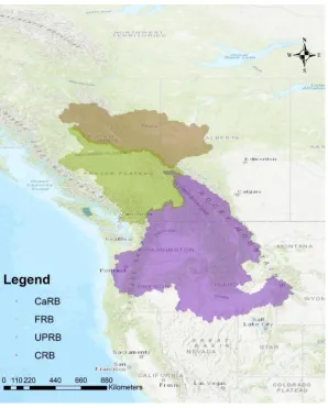
Figure 2. Four key river basins in WNA (light green: FRB, beige: PRB, purple: CRB, blue: CaRB)

This study analyzes the hydroclimatic extreme events and determine their relationship with

large-scale climate variabilities over four key basins in Pacific Northwest (FRB, UPRB, CRB

and CaRB) covering more than 958 thousand square kilometers (Figure 2). Not only the area

is so large to use high-resolution data for, but also the elevation varies a lot within the study

area, which makes the precipitation and temperature over the study area fluctuated.

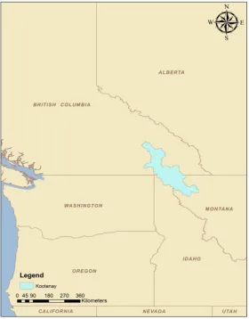
Moreover, the impact of climate change on streamflow is assessed over the Kootenay

(Kootenai) River Basin (KRB). The KRB (Figure 3) is a major river basin in southeastern

British Columbia and northern Montana and Idaho in the United States. The KRB, whose outlet

is Skookumchuck, is the second largest tributaries of the Columbia River. The length of KR is

(40)

22

Rockies with the mean elevation of 1800 meters. The KRB is divided into three sub-watersheds

draining approximately 13000 km2. The range of temperature is from below freezing in winters

to 30 °C in summers. The annual peak flows of the KRB exceed 660 m3/s routinely.

Figure 3. Kootenay River Basin

3.2. Data

The analyses are conducted using high-resolution observations and simulations at 1/16° spatial

and daily temporal resolution. This section describes downscaled data, gridded observations,

(41)

23

3.2.1. Daily Gridded Observation

Daily gridded observed precipitation, Max/Min temperature at 1/16° spatial and daily temporal

resolution are provided by the hydrology team at the Pacific Climate Impacts Consortium

(PCIC) that covers 1951-2010. Observation dataset is obtained in NetCDF (*.nc) file format

and is accessed and analyzed using R statistical programming language.

3.2.2. General Circulation Models

Hydroclimatic extremes are influenced by internal variability, natural (e.g. changes in solar

radiation, volcanic eruptions) and anthropogenic forcing factors (e.g. increases in GHG

concentrations including CO2, CH4 etc.). General Circulation Models (GCMs) are complex

atmosphere-ocean-land numerical models that are commonly used to understand changes of

extreme events in response to human-induced climate change and the role of internal

variability/forcing response and predict projected changes in hydroclimatic variables in the

future. We use a set of GCM simulations that participated in the Coupled Model

Intercomparison Project Phase 5 (CMIP5) (Meehl et al., 2000). In addition, we use a large set

of simulations (50 ensemble runs) from a single GCM (i.e. CanESM2) to better understand the

uncertainties in model structures and initialization, the role of internal variability and forcing

response in hydroclimatic extremes of WNA, and predict the projected changes of extreme

events (Tebaldi and Knutti, 2007; Tebaldi, Arblaster and Knutti, 2011; Deser, Knutti, Solomon

(42)

24

GCM Downscaling

GCMs contain large-scale information of the hydroclimate system (including forcing responses

and internal variabilities), however they have a coarse spatial resolution and cannot be used to

analyze hydroclimatic extremes at local scales particularly in regions with complex topography

(Mearns et al., 2001). Downscaling, which is the process of translating coarse resolution GCM

simulation outputs to regional hydroclimatic variables at fine spatiotemporal resolution, is

commonly categorized into two approaches: statistical downscaling and dynamical modeling

(Haylock et al., 2006; Najafi, Moradkhani and Wherry, 2011). In dynamical downscaling,

Regional Climate Models (RCMs) are nested within GCMs to represent the historical/future

physical processes at a high resolution (Christensen and Christensen, 2004; Pal, Giorgi and Bi,

2004; Frei et al., 2006; Fowler et al., 2007; Wood et al., 2004). This approach is

computationally demanding and can be time consuming. The other drawback of dynamical

downscaling is the dependency of RCMs on boundary conditions obtained from GCMs and

lack of transferability to different regions (Mandal, Srivastav and Simonovic, 2016).

Statistical downscaling methods find empirical linear/nonlinear relationships between large

scale predictors (i.e. GCM outputs) and local scale predictands (e.g. local precipitation) using

a variety of statistical techniques (Wilby and Wigley, 1997). One of the advantages of statistical

downscaling is its simplicity and flexibility (requiring relatively straightforward modifications

for use at various locations) compared to dynamical downscaling approach. Which has made

it popular among researchers.

In this study, we used GCM simulations that are downscaled statistically using a

state-of-the-art method called Bias Correction/Constructed Analogues with Quantile mapping reordering

(43)

25

Correction Constructed Analogues (BCCA) with Bias Corrected Climate Imprint delta method

(BCCI) and is suitable for the analysis of extreme events (Cannon, Sobie and Murdock, 2015).

CMIP5 GCMs

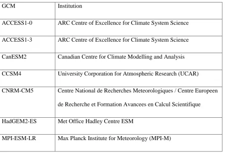
We analyzed outputs from seven CMIP5 GCMs (including precipitation, minimum and

maximum temperature) for historical (1981-2010) and future (2060-2089) time periods, which

include ACCESS1-0, ACCESS1-3, CanESM2, CCSM4, CNRM-CM5, HadGEM2-ES, and

MPI-ESM-LR (Table 2). All GCMs are downscaled using the BCCAQ approach based on the

Representative Concentration Pathway (RCP)8.5 (Werner and Cannon, 2016).

Table 2.GCMs used in this study

GCM Institution

ACCESS1-0 ARC Centre of Excellence for Climate System Science

ACCESS1-3 ARC Centre of Excellence for Climate System Science

CanESM2 Canadian Centre for Climate Modelling and Analysis

CCSM4 University Corporation for Atmospheric Research (UCAR)

CNRM-CM5 Centre National de Recherches Meteorologiques / Centre Europeen

de Recherche et Formation Avancees en Calcul Scientifique

HadGEM2-ES Met Office Hadley Centre ESM

(44)

26

CanESM2 Large Ensemble (LE) Simulations

A large ensemble of 50 climate simulations based on the CanESM2 model (CanESM2-LE) are

used to distinguish the uncertainties in model structure and internal variability and assess the

roles of forcing responses and variability in regional hydroclimatic extremes. These

simulations represent changes in the initialization of the CanESM2 GCM. Hence, the modeling

uncertainty boundary would cut off due to the unit structure of the simulation model. Similar

to other GCMs, we used downscaled precipitation, minimum and maximum temperature over

the historical (1981-2010) and future (2060-2089) periods. The Large Ensemble simulations

have been downscaled by PCIC to 1/16° resolution using BCCAQ under the RCP8.5 emission

scenario (Werner and Cannon, 2016).

All datasets are obtained in *.nc file format and are accessed and analyzed using R statistical

programming language.

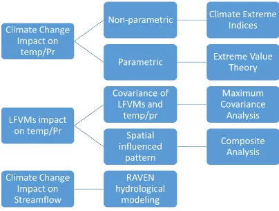
3.3. Methods

The statistical and process-based models to assess the impacts of climate change and LFVMs

on hydroclimatic extremes in WNA are described in this section, which include: climate

extreme indices, Generalized Extreme Value distribution, composite analysis, maximum

covariance analysis and hydrological modeling. Figure 4 briefly demonstrates the flowchart of

(45)

27

Figure 4. Methodology flowchart

3.5.1. Climate extreme indices

Climate extreme indices (i.e. CLIMDEX) were defined by Expert Team on Climate Change

Detection and Indices (ETCCDI). Most of these indices represent moderate extremes that occur

at least once a year (Zhang et al., 2011). There are 27 CLIMDEX indices available that are

based on daily data from which 16 are temperature-based and 11 are precipitation-based. Some

indices can be used to estimate hydroclimatic extremes with long return periods using annual

(46)

28

CLIMDEX can be divided into two categories. One that characterizes the amounts of

maximum/minimum temperature and precipitation and the other that measure the number of

days in a year when extremes exceed certain threshold (Zhang et al., 2011). Analysis of both

types of indices are critical for the design and planning of structure and infrastructure,

agricultural and water resources management. Through a comprehensive literature review, we

selected eight indices that best represent the intensity and frequency of extreme temperature (3

indices) and precipitation (5 indices)(Karl, Nicholls and Ghazi, 1999b; Zhang et al., 2005).

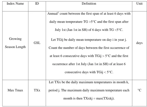
These indices are described in Table 3.

Table 3.Climate extreme indices (CLIMDEX) that are analyzed in this study

Index Name ID Definition Unit

Growing

Season Length

GSL

Annual1_{count between the first span of at least 6 days with}

daily mean temperature TG >5°C and the first span after

July 1st (Jan 1st in SH) of 6 days with TG <5°C.

Let TGij be daily mean temperature on day i in year j.

Count the number of days between the first occurrence of

at least 6 consecutive days with TGij > 5°C and the first

occurrence after 1st July (Jan 1st in SH) of at least 6

consecutive days with TGij < 5°C.

days

Max Tmax TXx

Let TXx be the daily maximum temperatures in month k,

period j. The maximum daily maximum temperature each

month is then TXxkj = max(TXxkj).

°C

1_{Annual means Jan 1st to Dec 31st in the Northern Hemisphere (NH); July 1st to June 30}th_{in the Southern}

(47)

29

Min Tmin TNn

Let TNn be the daily minimum temperatures in month k,

period j. The minimum daily minimum temperature each

month is then TNnkj=min(TNnkj)

°C Number of Heavy Precipitation Days R10

Let RRij be the daily precipitation amount on day i in

period j. Count the number of days where RRij ≥ 10mm

days

Max 5-day

Precipitation

Amount

RX5day

Let RRkj be the precipitation amount for the 5-day interval

ending k, period j. Then maximum 5-day values for period

j are Rx5dayj = max (RRkj)

mm

Simple Daily

Intensity Index

SDII

Let RRwj be the daily precipitation amount on wet days, w

(RR ≥ 1mm) in period j. If W represents number of wet

days in j, then:

𝑆𝐷𝐼𝐼_𝑗 =∑ 𝑅𝑅𝑤𝑗

𝑊 𝑤=1

𝑊

mm/day

Very Wet Days R95pTOT

Let RRwj be the daily precipitation amount on a wet day w

(RR ≥ 1.0mm) in period i and let RRwn95 be the 95th

percentile of precipitation on wet days in the 1961-1990

period. If W represents the number of wet days in the

period, then:

𝑅95_{𝑝𝑇𝑂𝑇} = ∑ 𝑅𝑅_𝑤𝑗

𝑊

𝑤=1

𝑤ℎ𝑒𝑟𝑒 𝑅𝑅_𝑤𝑗 > 𝑅𝑅_𝑤𝑛95