Role of Indigenous Knowledge in Mitigation and Adaptation to Climate Variability Impacts on Coastal Settlement Areas in Mombasa County, Kenya

(1)

ROLE OF INDIGENOUS KNOWLEDGE IN MITIGATION AND ADAPTATION TO CLIMATE VARIABILITY IMPACTS ON COASTAL

SETTLEMENT AREAS IN MOMBASA COUNTY, KENYA

By

SHERIFF, SALIA S. (BSc. Chemistry) Reg. No: N50F/CTY/PT/33185/2015

A Research Project Report Submitted in Partial Fulfillment of the Requirements for the Award of the Degree of Master of Environmental Studies (Climate Change and Sustainability) in the School of Environmental Studies in Kenyatta University

(2)

ii

DECLARATION Declaration by Candidate

This Project is my original work and has not been presented for a degree in any other university.

Name: SHERIFF, SALIA S.

Reg. No: N50F/CTY/PT/33185/2015

Signature… ………

Declaration by Supervisor:

This project has been submitted for examination with my approval as the University supervisor.

Supervisor:

Name: Dr. James Koske (PhD)

(3)

iii

DEDICATION

(4)

iv ABSTRACT

(5)

v

TABLE OF CONTENT

DECLARATION ... ii

DEDICATION ... iii

LIST OF TABLES ... viii

LIST OF FIGURES ... x

LIST OF ACRONYMS AND ABBREVIATIONS ... xi

CHAPTER ONE: INTRODUCTION ... 1

1.1 Background of the Study ... 1

1.2 Statement of the Problem ... 2

1.3 Research Questions ... 3

1.4 Research Objectives ... 3

1.5 Hypothesis ... 4

1.6 Justification ... 4

1.7 Conceptual Framework ... 5

1.8 Definitions of Terms ... 6

CHAPTER TWO: LITERATURE REVIEW ... 7

2.1 Climate Change Overview ... 7

2.2 Climate Science and Society ... 8

2.3 Indigenous Knowledge and Climate Change ... 9

2.4 Sea Level Rise and Flooding ... 9

2.5 Isolation of Knowledge Gaps ... 11

CHAPTER THREE: METHODOLOGY ... 12

3.1 Study Area ... 12

3.2 Research Design ... 12

3.3 Population ... 13

3.4 Sampling Procedures and Sample Size ... 13

3.5 Research Instruments ... 14

3.6 Data Collection ... 14

3.7 Data Analysis ... 15

CHAPTER FOUR: DATA PRESENTATION AND ANALYSIS ... 16

4.1 Introduction ... 16

4.2 Respondents Demographics ... 16

4.1.1 Gender of Respondent ... 17

4.1.2 Age of Respondents ... 18

(6)

vi

4.1.4 Household Size of Respondents ... 21

4.1.5 Occupation of Respondents ... 22

4.2 Variation in Temperature and Rainfall (Climate Variability) ... 24

4.2.1 Temperature ... 24

4.2.2 Rainfall ... 27

4.3 Effect of Sea Level Rise on Communities in Study Area for Past 30 Year. ... 31

4.3.1 Effects of Flood on Income ... 31

4.3.2 Estimated Damage of Flood ... 32

4.3.3 Occurrence of similar-flood causing damages ... 33

4.3.4 Benefit of Fresh and Salt water ... 34

4.3.5 Perception on the Causes of Flooding ... 34

4.3.6 Frequency of Flood ... 35

4.3.7 Hypothesis Testing for Effect of Sea-level Rise Variables... 36

4.4 Role of Environmental Education on Flood Impact Adaptation and Mitigation as Results of Sea Level Rise. ... 39

4.4.1 Knowledge on Flood Prediction ... 39

4.4.2 Reliability of the Knowledge ... 40

4.4.3 Challenges to Good Flood Prediction ... 40

4.4.4 Distance of Respondents’ Livelihood from River-bank/Seashore ... 41

4.4.5 Hypothesis Testing for Role of Environmental Education Variables ... 42

4.5 Community Preparedness to Climate Change Related Disasters Using Indigenous Knowledge ... 46

4.5.1 Flood training in Community ... 46

4.5.2 Local Practice ... 47

4.5.3 Flood Resilience ... 52

4.5.4 Flood Diseases and Prevention Methods ... 52

4.5.5 Hypothesis Testing for Community Preparedness Variables ... 54

4.6 Socio-Economic Impact of Climate Change ... 58

4.6.1 Impact of flood on settlement ... 58

4.6.2 Efforts to Increase Climate Change Awareness ... 59

4.6.3 Sea Level Rise Impact on Income... 59

4.6.4 Causes of Sea Level Rise Impact on Income ... 60

4.6.5 Hypothesis Testing for Socio-Economic Effect Variables ... 61

(7)

vii

CHAPTER FIVE: SUMMARY, CONCLUSIONS AND RECCOMENDATIONS

... 68

5.1 Summary ... 68

5.2 Conclusions ... 70

5.3 Recommendations ... 71

5.4 Suggestion for further studies ... 72

REFERENCES ... 1

APPENDICES ... 10

(8)

LIST OF TABLES

TABLE 4.1:SUMMARY SAMPLE OF RESPONDENTS ... 17

TABLE 4.2:GENDER SUMMARY OF RESPONDENTS ... 17

TABLE 4.3:AGE SUMMARY OF RESPONDENTS. ... 19

TABLE 4.4:LEVEL OF EDUCATION OF RESPONDENTS. ... 20

TABLE 4.5:HOUSEHOLD SIZE OF RESPONDENTS. ... 21

TABLE 4.6:OCCUPATION OF RESPONDENTS ... 23

TABLE 4.7:ANOVA SINGLE FACTOR TEST SUMMARY FOR TEMPERATURE ... 26

TABLE 4.8:ANOVA SIGNIFICANCE TEST FOR TEMPERAURE ... 27

TABLE 4.9:ANOVA SINGLE FACTOR TEST SUMMARY FOR RAINFALL ... 30

TABLE 4.10:ANOVA SIGNIFICANCE TEST FOR RAINFALL ... 31

TABLE 4.11:FLOOD EFFECT ON RESPONDENTS' INCOME ... 32

TABLE 4.12:RESPONDENTS' ESTIMATED DAMAGE CAUSED BY FLOOD ... 33

TABLE 4.13:RESPONDENTS' FREQUENCY ESTIMATED DAMAGE CAUSED BY FLOOD. ... 33

TABLE 4.14:RESPONDENTS' BENEFIT FROM FRESH AND SALT WATER FLOODS. ... 34

TABLE 4.15:RESPONDENTS' PERCEPTION ON FLOODING ... 35

TABLE 4.16: FREQUENCY OF FLOODING ... 36

TABLE 4.17:DEPENDENT VARIABLE FOR SEA LEVEL RISE HYPOTHESIS ... 36

TABLE 4.18: SEA LEVEL RISE VARIABLES NOT IN THE EQUATION ... 37

TABLE 4.19:SEA LEVEL RISE VARIABLE IN THE EQUATION ... 37

TABLE 4.20:RESPONDENTS' PREDICTION ON THE OCCURRENCE OF FLOOD ... 39

TABLE 4.21:RELIABILITY OF RESPONDENTS' PREDICTION ON THE OCCURRENCE OF FLOOD . 40 TABLE 4.22:CHALLENGES TO RESPONDENTS' PREDICTION ON THE OCCURRENCE OF FLOOD 41 TABLE 4.23:RESPONDENTS' ACTIVITY DISTANCE FROM RIVERBANK AND SEASHORE ... 42

TABLE 4.24:DEPENDENT VARIABLE FOR THE ROLE OF ENVIRONMENTAL EDUCATION HYPOTHESIS ... 43

TABLE 4.25:ROLE OF ENVIRONMENTAL EDUCATION VARIABLES NOT IN THE EQUATION ... 44

TABLE 4.26:INDEPENDENT VARIABLES FOR THE ROLE OF ENVIRONMENTAL EDUCATION HYPOTHESIS ... 45

TABLE 4.27:RESPONDENTS' TRAINING ON FLOOD ... 46

TABLE 4.28:RESPONDENTS' LOCAL PRACTICE TO PREVENT FLOOD ... 48

TABLE 4.29:RESPONDENTS' PERCEPTION ON PROPER PRACTICE TO REDUCE FLOODING ... 49

(9)

ix

TABLE 4.31:RESPONDENTS' PERCEPTION TO ENHANCING FLOOD RESILIENCE ... 52

TABLE 4.32:DEPENDENT VARIABLES FOR COMMUNITY PREPAREDNESS HYPOTHESIS ... 54

TABLE 4.33:COMMUNITY PREPAREDNESS VARIABLES NOT IN THE EQUATION ... 56

TABLE 4.34:INDEPENDENT VARIABLES FOR COMMUNITY PREPAREDNESS HYPOTHESIS ... 57

TABLE 4.35:DEPENDENT VARIABLES FOR SOCIO-ECONOMIC EFFECT HYPOTHESIS ... 61

TABLE 4.36:SOCIO-ECONOMIC EFFECT VARIABLES NOT IN THE EQUATION ... 62

TABLE 4.37:INDEPENDENT VARIABLES FOR SOCIO-ECONOMIC EFFECT HYPOTHESIS ... 62

TABLE 4.38:SUMMARY OF RESPONDENTS IN THE BLR ... 64

TABLE 4.39:VALUE OF DEPENDENT VARIABLE ... 65

TABLE 4.40:BLR CLASSIFICATION TABLE ... 65

TABLE 4.41:EQUATION VARIABLE ... 66

(10)

LIST OF FIGURES

FIGURE 1.1:CONCEPTUAL FRAMEWORK. ... 5

FIGURE 1.2:STUDY AREA, ADOPTED FROM THE MINISTRY MINING,KENYA,2012. ... 12

FIGURE 4.1: RESPONDENTS INDIGENOUS KNOWLEDGE AND GENDER ... 18

FIGURE 4.2:RESPONDENTS'INDIGENOUS KNOWLEDGE AND AGE ... 19

FIGURE 4.3:RESPONDENTS' INDIGENOUS KNOWLEDGE AND LEVEL OF EDUCATION ... 21

FIGURE 4.4:RESPONDENTS'INDIGENOUS KNOWLEDGE AND HOUSEHOLD SIZE... 22

FIGURE 4.5:RESPONDENTS' INDIGENOUS KNOWLEDGE AND OCCUPATION ... 23

FIGURE 4.6:MEAN MONTHLY TEMPERATURE (1984-2014) ... 24

FIGURE 4.7:TOTAL ANNUAL TEMPERATURE (1984-2014) WITH 5 YR. MOVING AVERAGE ... 25

FIGURE 4.8:TEMPERATURE VARIABILITY FROM LONG TERM MEANS (1984-2014) ... 25

FIGURE 4.9:MEAN TEMPERATURE OVER 10 YR. PERIOD ... 26

FIGURE 4.10:MONTHLY RAINFALL (1986-2014)AVERAGE ... 28

FIGURE 4.11:TOTAL ANNUAL RAINFALL (MM) FOR MOMBASA (1986-2014) ... 28

FIGURE 4.12:RAINFALL VARIABILITY FROM LONG TERM MEANS 987MM)1986-2014. ... 29

FIGURE 4.13:MEAN RAINFALL OVER 10YR. PERIOD. ... 30

FIGURE 4.14:FREQUENT DISEASE DURING FLOODING PERIOD. ... 53

FIGURE 4.15:RESPONDENTS'MALARIA PREVENTION METHODS. ... 53

FIGURE 4.16:RESPONDENT'S CHOLERA PREVENTION METHODS. ... 54

FIGURE 4.17:IMPACT OF FLOODING ON RESPONDENTS' SETTLEMENT. ... 58

FIGURE 4.18:RESPONDENTS' PERCEPTION ON COMMUNITY EFFORT TO INCREASE CLIMATE CHANGE AWARENESS. ... 59

FIGURE 4.19:GRAPH SHOWING SEA LEVEL RISE EFFECT ON RESPONDENTS' SOURCE OF INCOME. ... 60

(11)

LIST OF ACRONYMS AND ABBREVIATIONS B Bamburi ward as indicated in Tables BLR Binary Logistics Regression

CCC California Coastal Commission

CH4 Methane

CNRA California Natural Resources Agent

CO2 Carbon Dioxide

DEM Digital Elevation Model

GDP Gross Domestic Product

GHG Greenhouse Gas

GoK Government of Kenya

IPCC Intergovernmental Panel on Climate Change J Junda ward as indicted in Tables

K Kissimini ward as indicated in Tables KARI Kenya Agricultural Research Institute M Magogoni ward as indicated in Tables

N Population Size

n Sample Size

N2O Nitrous Oxide

PR Port Reitz ward as indicated in Tables

(12)

xii

SPSS Statistical Package for Social Scientists

(13)

i

CHAPTER ONE: INTRODUCTION 1.1 Background of the Study

Intensified coastal flooding, coastline erosion, and marshland vulnerability are highly influenced by sea level rise. These wetlands (marshlands) enhance flood reduction, carbon sequestration, improve water quality, and widen marine and wildlife habitats ( Wigand, Ardito, Chaffee, Ferguson, Paton, Raposa, and Watson, 2017). Coastal populations have continuously benefited from the enormous ecosystem services provided by coastal wetlands despite their vulnerabilities to Sea Level Rise. However, human activities are largely responsible for rapid Sea Level Rise and its impacts on the socio-economic lives on adjacent uplands (Kirwan and Megonigal, 2013). The fight to combat the present and future impacts of climate change and climate variability is a global goal. The challenges are huge on developing countries especially the ones having densely populated cities along the coastal areas. Rising Sea level, low-lying areas, extreme weathers and excessive water levels are potential threats that amplify the risks of the impacts to human beings. The impacts are more profound in economic coastal zones and unplanned cities, (McGranahan, Blak, and Anderson, 2007). Though coastal flood losses and adaptation costs consequential from sea level rise of the 21th century are evaluated globally considering several factors such as inconsistence in continental based data, demographic data, protection approaches, and socioeconomic development ( Hinkelet al., 2014). The extent of these impacts varies amongst places according to local or regional climates, geological movements and anthropogenic activities which contribute to land use changes. However, record shows that there is little knowledge about rising sea level and climate change impacts including coastal problems in Africa from the limited access to climate-related data. This is especially so due to the limited technological and institutional capacity, low economic development and abject poverty (Zinyoweraet al., 2009).

(14)

2

population and geographic ranges (Confalonieri et al., 2007). This could also affect productivity and efficiency in densely human population in urban areas. In this regard, it is important to increase adaptation capacity alongside mitigation efforts; because it is estimated that increasing mitigation alone will swiftly better climate in this century. Therefore, effective adaptation is indivisibly required to lower the impacts of already occurring (IPCC, 2013; Stein et al., 2013).

In coastal areas, climate change related impacts could be pronounced as result of Sea Level Rise (SLR). This will increase property damage consequently from inundation, flooding, erosion, high waves, loss of beaches and recreation centers, and loss of ecologically important wetlands (Heberger Cooley, Herrera, Gleick, and Moore, 2009). Other impacts include damaging of public infrastructures such as wastewater treatment facilities, low-lying roads, piers, ports, and facilities located on coastal bluffs. Even though a benefit of SLR could be lesser need for dredging, but until such facilities make available spaces for large ships than they presently have, increase sea levels pose serious challenge for cargo delivery (California Coastal Commission, 2001; CNRA, 2014). Efforts at local and international levels are required to mitigate climate variability and climate change risks. These efforts include an effective climate risks management system that requires national framework and institutions, access to effective and efficient climate data and information, adequate human capacity, advanced technology, and financial resources (Hellmuth et al., 2007). In Kenya, increasing climate variability and the projected rise in global mean air and sea temperatures, sea level and precipitation including varying frequency and severity of extreme weathers would have substantial implications on the socioeconomic and environmental structures in the country (GoK, 2015). Increase in sea surface temperature and marine biological invasion such as invasive species and harmful algal blooms affect the coral reef ecosystems. This would negatively impact the livelihoods of millions of people in the region who dependent on this ecosystem for food, income, and shoreline defense (GoK, 2015).

1.2 Statement of the Problem

(15)

3

reports from many multilateral environmental agreements. Despite these policies, many local people have no formal knowledge on climate change and its anthropogenic causes, but they have mutually benefited from their imperial knowledge on climate change variability to survive for many centuries ago. In view of this, it is very necessary to put local indigenous knowledge at the fulcrum of environmental sustainability decision making especially for the growing coastal settlements in Africa in order to mitigate climate change and climate variability impacts to pave the ways for the achievements of a clean environment for all. In Kenya, particularly the coast, local traditional knowledge and belief system have drawn little national and international attention to address climate variability impacts. Therefore, it is paramount to carry out research and get understanding of local indigenous knowledge and practices and impact on climate variability in the coastal settlements.

1.3 Research Questions

i. How has climate (rainfall and temperature) varied in the research area between 1986 and 2016?

ii. Is climate variability associated with sea level rise and flooding in Kisauni, Nyali, and Changamwe?

iii. What impact does climate variability have on community livelihoods?

iv. How do communities in Port Reitz, Tudor, Magogoni use indigenous knowledge to mitigate and adapt to climate change impact?

v. How do socio-economic factors influence the application of indigenous knowledge in adaptation and mitigation of climate change impacts in the study areas?

1.4 Research Objectives

The general objective of this study was to investigate Indigenous Knowledge and its mitigation and adaptation measures to flooding and climate variability impacts in Mombasa County, Kenya. The specific objectives include:

i. To determine the variation in temperature and rainfall (climate variability) between 1986 and 2016.

(16)

4

iii. To understand the role environmental education has played in shaping communities’ indigenous adaptation capacity and mitigation measures in coping with flooding as results of sea level rise.

iv. To assess the level of preparedness of these communities to cope with climate change related disasters through application of indigenous knowledge in adaptation and mitigation of climate change impacts

v. To determine how socio-economic impact of climate change affect people in the study areas.

1.5 Hypothesis

H1: The five alternative hypotheses are stated below:

i. There is significant variation in temperature and rainfall (climate variability) between 1986 and 2016.

ii. Sea level rise as a result of climate change significantly affects the communities. iii. Low environmental education is statistically significant and influences

communities’ indigenous flood-adaptation and coping measures.

iv. Low level of community preparedness to flood is statistically significant and influences the application of indigenous flood-adaptation and coping measures. v. Climate change significantly has socio-economic impacts on the communities.

1.6 Justification

(17)

5 1.7 Conceptual Framework

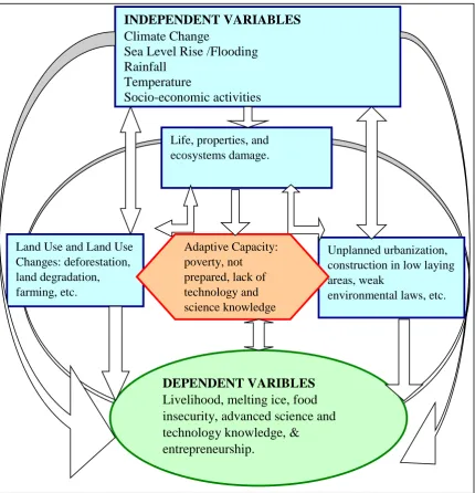
The research was focused on flooding in Mombasa County as the result of climate variability phenomena and how local communities in the study areas have coped with such impacts. In this regard, the conceptual framework focuses on climate induced tools that influence regional climate variables and consequently leads to flooding and other weather phenomena.

Source: adopted from Maureen and Clare, (2016).

INDEPENDENT VARIABLES 1. Climate Change

2. Sea Level Rise /Flooding 3. Rainfall

4. Temperature

5. Socio-economic activities

Life, properties, and

ecosystems damage.

Land Use and Land Use Changes: deforestation, land degradation, farming, etc.

Unplanned urbanization, construction in low laying areas, weak

environmental laws, etc.

DEPENDENT VARIBLES Livelihood, melting ice, food insecurity, advanced science and technology knowledge, & entrepreneurship.

Adaptive Capacity: poverty, not prepared, lack of technology and science knowledge

(18)

6 1.8 Definitions of Terms

Climate Change: refers to the changes in the mean weather condition of the study area and others places around the world about decade or longer, (GoK, 2009).

Climate Variability: refers to the meteorological changing in the climate of the weather of the study areas and other in stations around the world often annually, (Hageback et al., 2005).

Community: this refers specifically to geographically defined places and groups of people living close to one another within the study communities, i.e., Port Reitz, Junda, Bamburi, Mogongo, and Kissimani in Mombasa County where the study will be conducted, (Shilabukha, 2015).

Exposure: this tells the likelihood and possibility of communities in the coastal areas that would be affected by bad climate variability and climate change effects such flooding and storms due to low coping capacity (unpreparedness), (Kebede et al., 2009). Farming: refers mainly to low income farming (sustenance) that includes cropping, animal husbanding, and fishing in the study areas, (Sakane et al., 2013).

Flooding: this refers to over flooding of the creeks and rivers in the study areas resulting from sea level rise, hence causing human displacement, disrupting farming and other commercial activities (Awuor et al., 2008: Kebede et al., 2009).

Impact: this is the consequential and harmful effects coastal settlements experience whenever flooding occurs as result of Sea Level Rise and bad climate events (Kebede

et al., 2009).

(19)

7

CHAPTER TWO: LITERATURE REVIEW 2.1 Climate Change Overview

Climate change is believed to have exacerbated the present drought and its impacts-famine, loss of livestock, and lack of potable water in Kenya and some other places in East Africa (Briefing, 2017). It is considered worst drought in recent decades in the sub region (Firebrace, 2016). In many different aspects, the drought has damaging impacts than the 2010/2011 food crisis that affected millions of people because it is the consecutive year of largely characterized by low in addition to high temperature (OCHA, 2017). This trend is bent curved to the IPCC reports of expected increasing climate change impacts to Kenya and others developing as result of low coping capacity (IPCC, 2014). It is anticipated that temperature increases, for example, in the Himalayas may disturb timing and amount of precipitation that would impact water availability that region (Mishra, Babel, and Tripathi, 2014).

(20)

8

Although earth’s climate always changes as a result of interactive forcing amongst its components: hydrosphere, biosphere, cryosphere, and atmosphere but the changes experienced from the past century are unprecedented. These changes are widely accepted to be induced by human activities (Pachauri and Reisinger, 2007). Combustions of carbon-based fuels in industries, transportations (motor vehicles, ships, trains, and aero planes) and energy sectors (generators, coals, etc.) over the past century has increased CO2 concentration in the atmosphere and the global mean temperature by 368 ppm and 0.74 0C respectively, by 2000 (Watson, 2001). These figures are projected to further increase to 1250 ppm and 3.4 0C by 2095. This higher increase will go along with greater climate variability and extreme events (Flooding, drought, heat and cold waves, etc.) (Pachauri and Reisinger, 2007).

2.2 Climate Science and Society

In places like the Maldives, where sea level rise is predicted to cause mass migration local communities do consider sea level rise a major factor affecting their communities and livelihoods (Robert et al., 2017). In addition, projections that lowland country of such kind are obtained from high solution spatial and temporal simulation models that provide difference in regional climate impacts. However, data show that regional and seasonal difference in model simulations do not account for the physical implications such climates will cause on living organisms such as humans, crop sowing, vectors, pathogens, pests infections, and distributions (Barnett et al., 2006). Thus, the determination of climate change and global warming impacts is highly subjective. For example, Sea Level Rise is believed to have occurred about few meters than it is in present days (Heartyet al., 2007; Dutton and Lambeck, 2012). Further geologic assessments of the shorelines have confirmed that eustatic sea level rise as high as 9 meters above the present towards the last interglacial. This proposes that a critical ice sheet stability a brink has been crossed which caused the breakdown of polar ice sheet and substantial sea level rise (O’Learyet al., 2013).

These finding simply imply that significant ice sheet melting occurred when the earth was a little warmer than it is today.

(21)

9

Nicholls et al., 2007b). A little increased in sea level can cause significant impacts such as flooding, erosion, extreme weather events and saltwater intrusion (Nicholls et al., 2007a; Bicknell et al., 2009). Thus, the impacts vary from one region to another in relation to its geography.

2.3 Indigenous Knowledge and Climate Change

As the conducting body of climate change mitigation and adaptation action plans, the intergovernmental panel on climate change (IPCC) mentioned in its fifth assessment report that little efforts have been applied to fully incorporate indigenous knowledge into its reports; hence under representing the critical roles and values culturally relevant and appropriate adaptation measures that need a vigorous inclusion suitably (Ford, Cameron, Rubis, Maillet, Nakashima, Willox and Pearce, 2016) . A study carried out amongst the Giriama people of North Coast (Kenya) demonstrated that their use of indigenous knowledge and traditional management practices exemplified through their systems of naming, taboos, common sayings, and life-long experiences have jointly contributed to the sound environmental supervision of mangroves, fisheries, corals and coral reefs conservations (Shilabukha, 2015). Indigenous knowledge, an embodiment of knowledge, belief and practices including one’s inter personal relationships and interaction with his/her surrounding environments that have evolved amongst a group of people through adaptation and transfer between generations (Berks, 1993). This means, every community has got some unique practices to sustainably interact and preserve its ecological diversity (Patnaik, 2002). An evaluation of the contributions of indigenous knowledge of Native American Indian of Alaska to climate change adaption strategies and their worldviews of climate change emphasizes the invaluable roles to lessen climate impacts. This is not limited to Native American Indians, but to other native communities of the world in their localities. In this regards, it called for an uncompromising teaming of native scholars, community leaders, and scientist including policymakers to find more sustainable and diverse solutions to climate change response challenges (Shilabukha, 2015).

2.4 Sea Level Rise and Flooding

(22)

10

estimated to be submerged by 17% with a 30 cm rise in sea level (Awuor, Orindi, and Adwera, 2008). Flooding is one of the frequent natural disasters experience in major coastal cities, from western to coastal Kenya. There are varying benefits and consequences regionally (Brown, Nicholls and Lowe, 2016). Mombasa, the largest seaport in Kenya has beautiful marine attractions and beaches including geographic landmarks and conversancy, making Kenya’s most visited county (e.g. Mohamed, 2009). The history of unusual climate events such as flooding is frequent, example in 2006; about 60,000 people in Mombasa were affected by flooding (Awuor et al., 2008). Mombasa County remains highly vulnerable to climate change; three geographic factors contributing to its vulnerability include high temperature, low altitude, and humidity. It located on coastal plain about 4-6 kilometer (Km) likely to be submerge by sea level rise causing complete disruption of ecosystem services, function and balance, interference with agricultural and industrial activities; hence damage human settlement and freshwater resources (GoK, 2002). This consequentially impacts the economy of Mombasa City and the Kenya at large.

Mombasa is strategically located; it founds an important pillar of national and regional economy of East Africa. The port city does not only serve Kenya but it neighboring landlocked countries including Burundi, Congo, Rwanda, South Sudan Tanzania and Uganda. It also attracts thousands of tourists owing to its terrestrial and marine ecological diversity. The beautiful beaches, warm weather, rich culture, and inherent historical sites and monuments are some stimuli to foreign tourists increasing the national foreign exchange and Gross Domestic Product (GDP) up to 12 percent in 2003 (GoK, 2006).

(23)

11

and economic growth will worsen as result of climate variability and change. Report of drought and increase water scarcity will high (UNEP, 2009). In the bottom-up approach to understanding climate variability and change impacts, local communities often provide crucial information to characteristics factors that strengthens or impedes the communities’ response, recovery and adaption. Therefore, it is important to incorporate local and indigenous knowledge in climate variability and change research design and implementation (Dolan and walker, 2003). Local and indigenous knowledge system plays a significant role in climate variability and change research. In a recent study, the Kenya Agricultural and Research Institute (KARI) recommended through a research it has conducted on the Kenyan Coast, the recording of the local and indigenous coping experience, strategy and resilience (Cenafrica., 2010).

2.5 Isolation of Knowledge Gaps

(24)

12

CHAPTER THREE: METHODOLOGY 3.1 Study Area

The study was conducted in five wards i.e., Junda, Bamburi, Magongo, kisimani, and Port Reitz in three constituencies, Kisauni, Nyali and Changamwe all in Mombasa County, Kenya. The samples were collected through the administering of research questionnaire and focused group discussion. The samples were analyzed using statistics.

Figure1.2: Study Area, (Ministry Mining, Kenya, 2012). 3.2 Research Design

(25)

13

The study was carried out using structured and semi-structured questions to the respondents/informants. The qualitative and quantitative data generated were analyzed separately using descriptive analysis (Leech and Onwuegbuzie, 2007).

3.3 Population

The target population of the study areas was about 939,370 people (GoK, 2009).The study focused on three constituencies within coastal Kenya, Mombasa that are settled along the Indian Ocean. In this regard, the study involved community residents of different professional and social backgrounds, heads of family, employees, farmers, and the business community, who are likely to be affected from the potential impacts of flooding including other related climate variability events from Junda, Bamburi, Magongo, Kisimani, and Port Reitz areas in Mombasa.

3.4 Sampling Procedures and Sample Size

The reliability of a scientific research depends on its representativeness of the population under study, i.e., adequate (larger) sample size is the true representation of the universe. However, the huge cost and time attached to large sample size is usually overwhelming for a purposeful research. Therefore, acceptable sample size determination techniques devised by researchers and scientists proven to be significant representation of a given population was used. The widely used Yamane’s formula as used in this research as expressed below (Yamane, 1967):

𝑛 = 𝑁 [1 + 𝑁∗_(𝑒)2_]

Where n =is the sample size, N=is the population size and e=is the acceptable sampling error. 95% confidence level with P=0.5 are assumed when using thesis formula. In this accord, the five communities comprising of about 155,638 people of the total population of the county is about 939, 370 people (Gok, 2009). Using the above formula, the total population of Mombasa County is 939,370, therefore the expected sample size is;

n= 939370/ [1+939370*(0.05)2] =399.829=400.

(26)

14

To representatively have a consistent data, the questionnaire was randomly administered to respondents in the research communities i.e., 99, 59, 66, 69, and 74 respondents from Junda, Bamburi, Magongo, Kisimani, and Port Reitz, respectively. There were also discussions with stakeholders from the county offices of the National Environmental Management Authority (NEMA) and the Kenya Meteorology Department (KMD) of Moi International Airport to get authorities’ views of Flood impacts and rainfall and temperature variability within Mombasa, respectively. The respondents were permanent residents who have stayed for about five years and more within the research areas. The sampling was sensitivity to gender and demographic distribution of the respondents.

3.5 Research Instruments

Structured and semi-structured questionnaires were used to collect adequate quantitative and qualitative data to for analysis. Secondary data was collected from the Kenya Metrological Department Mombasa substation, Moi International Airport for comparative correlation to primary field data to determine Climate Variability and its impacts. The questionnaires generated further information on loss of settlement and farm lands, interruption of viable economic activities, etc. due to flooding and sea level rise. The questionnaires were subdivided into: respondent’s demographic data, economic assessment, flood causes and impacts, community resilience to climate variability among other research objectives and goals.

3.6 Data Collection

(27)

15 3.7 Data Analysis

(28)

xvi

CHAPTER FOUR: DATA PRESENTATION AND ANALYSIS 4.1 Introduction

Variability of climate along coastal areas impacts the life style and economic activity of these local communities amidst global climate change emergency. It is therefore important to understand how these communities have seasonally been affected and how the indigenous people (permanent residents) from these communities adapt. On this backdrop, this study was aimed to assess the impacts of climate variability and the local indigenous adaptive and mitigation measures in Mombasa County. The local indigenous knowledge was studied through structured questions that assessed the respondents’ perceptions on the causes of climate variability and its impacts, the indigenous communities’ coping capacity and their local means of lowering climate variability impacts within the county. Mombasa county is hugely populated as result of its booming economic and frequent tourist visit. Part of the county is naturally a lowland area whereas other parts are densely occupied making the county vulnerable to the numerous impacts of flooding as result of sea level rise and heavy rainfall. In the test of hypotheses for objective 2, 3, 4 and 5: Binary Logistics Regression (BLR) was used as explained in details in section 4.7

4.2 Respondents Demographics

(29)

17 Table 4. 1: Summary of Sample of Respondents

Constituency Ward Total P (%)

Junda Bamburi Magogoni Kisimani Port Reitz

Kisauni 100 60 67 0 0 227 61.20

Nyali 0 0 0 70 0 70 18.90

Changamwe 0 0 0 0 74 74 19.40

Total 100 60 67 70 74 371 100

Source: Field Work (2017) 4.1.1 Gender of Respondent

Information necessary for this study was collected from 199 (54%) females, i.e., 54, 31, 35, 39 and 40 females from Junda, Bamburi, Magogoni, Kisimani, and Port Reitz, respectively (Table 4.2). In similar order, 172 (46%) males were sampled, 46, 29, 32, 31, and 34 giving a total of 371 respondents (Table 4.2).

Many disaster prevention and mitigation policy initiatives are not gender sensitive (UNISDR, 2012) and women are more likely to have higher fatality UNDP (2013). This study was sensitive to issues of gender as majority of the respondents were female, and thus an indication that the respondents were able to inform this research from a gender sensitive perspective as well.

Table 4. 2: Gender summary of Respondents

Gender Ward Total Percent

(%) Junda Bamburi Magogoni Kisimani Port

Reitz

Female 54 31 35 39 40 199 53.64

Male 46 29 32 31 34 172 46.36

Total 100 60 67 70 74 371 100

(30)

18

As shown in Figure 4.1, majority of the female respondents (47%) have no indigenous knowledge on flood prevention and mitigation. These findings are similar to those other studies which found that women’s ability to respond to flood is lower compared to men and their capacity to participate in flood management is low (Wiest, R.E., Mocellin, J.S.P. and Motsisi, D.T, 1994:13; Cannon, 2000:43-55; Few, R., Ahern, M., Matthies, F. & Kovats, S., 2004:25; Bhatti, 2001:16).

Figure 4.1: Respondents’ indigenous knowledge and by gender Source: Field Work (2017)

4.1.2 Age of Respondents

Out of the total respondents as shown in Table 4.3: 50% were adult (aged 36 to 59 years), 44% were youth (aged 21 to 35 years), and 3% each were adolescents and elderly. Within respective wards: majority of those in Junda and Kisimani were adults, while the majority in Bamburi, Magogoni and Port Reitz were youth. The number of adults as respondents is considerate enough to inform this study since they have more flood experience than the youth. Thus, outlining the findings of Kuhlicke (2006:14) that older persons have extensive knowledge about flooding.

0.0% 10.0% 20.0% 30.0% 40.0% 50.0%

No Yes

%

of

r

esp

on

d

en

ts

(31)

19 Table 4. 3: Age summary of respondents.

Age (Yrs.) Ward Total P(%)

Junda Bamburi Magogoni Kisi-mani

Port Reitz

18-20 Adolescent 0 0 4 1 5 10 2.70

21-35 Youth 10 32 44 32 44 162 43.66

36-59 Adult 82 27 16 37 24 186 50.14

60-Above Elderly 8 1 3 0 1 13 3.50

Total 100 60 67 70 74 371 100

Source: Field Work (2017)

As shown in Figure 4.2, most of the adult: about (44%) respondents have no knowledge about indigenous flood prevention and mitigation as compared to the youth (37%) while more of the youth (7%) have knowledge about indigenous flood prevention and mitigation than the adults (6%). Considering that the number of adults are more than the youth, and that the adult should be more experienced on indigenous management issues than the youth; this study found the opposite that the youth are more aware of indigenous prevention and mitigation flood measures. These findings agree with Bhatta (1999:24-25) findings that indigenous knowledge lacks accountability within communities; but disagrees with Bhatta that the lack of accountability is prevalent among the youth.

Figure 4.2: Respondents' Indigenous Knowledge by age Source: Field Work (2017)

0.0% 10.0% 20.0% 30.0% 40.0% 50.0%

18-20 Adolescence

21-35 Youth 36-59 Adult 60-Above Elderly

%

of

Re

sp

on

d

en

ts

(32)

20 4.1.3 Level of Education of Respondents

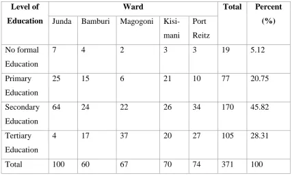
As shown in Table 4.4; 46% of the respondents were secondary school education, 28% has tertiary education, 21% has primary school education and 5% has no formal education. Within respective responses wards, majority of those in Junda, Bamburi, Kisimani, and Port Reitz have secondary education, while majority of those in Magogoni have tertiary education.

The respondents with both secondary and tertiary education account for 74%, this indicates that the respondents are knowledgeable enough to inform this study and able to increase their knowledge and understanding of climate variability and its predictable impacts. It is also agreed that education is important in understanding of climates change by the locals through their basic observation of temperature and precipitation (Adebayo, Dauda, Rikko, Fashola, Atungwu, Iposu, Shobowale, and Osuntade, 2011).

Table 4. 4: Level of education of respondents. Level of

Education

Ward Total Percent

(%) Junda Bamburi Magogoni Kisi-

mani

Port Reitz No formal

Education

7 4 2 3 3 19 5.12

Primary Education

25 15 6 21 10 77 20.75

Secondary Education

64 24 22 26 34 170 45.82

Tertiary Education

4 17 37 20 27 105 28.31

Total 100 60 67 70 74 371 100

(33)

21

with secondary have higher knowledge than those with primary; and those with primary have higher indigenous knowledge than those with no formal education.

Figure 4.3: Respondents' Indigenous Knowledge by Level of Education Source: Field Work (2017)

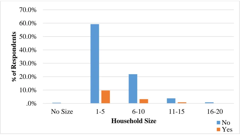
4.1.4 Household Size of Respondents

Table 4.5 shows 69% have household size of 1-5 persons, 25% have 6-10 persons in their household, and only 4% had a size of 16-20 persons. Across the wards, the majority of respondents have household size of 1-5.

Table 4. 5: Household Size of Respondents. Household

Size

Ward Total P(%)

Port Reitz

1-5 65 54 47 41 49 256 69

6-10 25 3 16 26 23 93 25.07

11-15 6 3 3 3 2 17 4.58

16-20 3 0 0 0 0 3 0.81

No Response

1 0 1 0 0 2 0.53

Total 100 60 67 70 74 371 100

Source: Field Work (2017) 0.0% 10.0% 20.0% 30.0% 40.0% 50.0% No formal Education Primary Education Secondary Education Tertiary Eduaction % of Re sp on d en ts

(34)

22

Figure 4.4 shows that 59% of those with no indigenous knowledge has 1-5 household size; and 22% of those with no indigenous knowledge has 6-10 household size. Also, 10% of the respondents that have indigenous knowledge has 1-5 household size while 4% of the respondents with indigenous knowledge has a household size of 6-10. This means that as household size increases above 5 persons the knowledge on indigenous flood prevention and management practices decreases. This shows that most of the respondents with lower household size, have more indigenous knowledge than those with higher household size.

Figure 4.4: Respondents' Indigenous knowledge and household size Source: Field Work (2017)

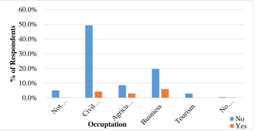
4.1.5 Occupation of Respondents

Out of the total respondents as shown in Table 4.6: majority (54%) were civil servants i.e. in the public or private service; 30% were in the tourism sector; 11% were in agricultural sector practicing crop farming, fishery and animal husbandry; 3% were engaged in the small-scale business sector; and 5% were unemployed. Within the wards: majority of those in Port Reitz were engaged in small scale businesses.

Close to half and considerable number of respondents are employed in the tourism, agriculture and small-scale business sector which makes them dependent on sources of livelihood that is more likely to be affected by climate variability.

.0% 10.0% 20.0% 30.0% 40.0% 50.0% 60.0% 70.0%

No Size 1-5 6-10 11-15 16-20

% o

f

Re

sp

on

d

en

ts

Household Size _No

(35)

23 Table 4. 6: Occupation of respondents

Occupation Ward Total P (%)

Port Reitz

Not employed 0 2 11 3 4 20 5.39

Civil Servant 83 42 25 28 21 199 53.63

Agriculture 3 7 12 2 19 43 11.59

Business 13 8 11 35 28 95 25.60

Tourism 1 1 6 2 1 11 2.96

No Response 0 0 2 0 1 3 0.80

Total 100 60 67 70 74 371 100

As shown in Figure 4.5, most of the respondents with no indigenous knowledge on the prevention and mitigation of floods are largely those in the civil service (49%) and business (20%) sector. However, fewer respondents in the agricultural sector (3%) have indigenous knowledge than those respondents in the civil service (4%) and business (6%) sector. This indicates that respondents of the critical sector which is tourism and agriculture, with the significance to make an impact on climate change are less impactful since they have no indigenous knowledge on flood mitigation and prevention.

Figure 4.5: Respondents' indigenous knowledge by occupation Source: Field Work (2017)

0.0% 10.0% 20.0% 30.0% 40.0% 50.0% 60.0%

%

of

Re

sp

on

d

en

ts

(36)

24

4.2 Variation in Temperature and Rainfall (Climate Variability)

Climate variations resulting especially from temperature and rainfall have the propensity to impact the settlers and adversely hinder their means of livelihood. 4.2.1 Temperature

From Figure 4.6, the data from KMD indicated that between 1984 and 2014, temperature was at its highest degree (420C) across the months of March; and at the lowest (280C) across the months of June, July and August.

Figure 4.6: Mean monthly temperature (1984-2014) Source: KMD Data (2017)

Between 1984 and 2014, temperature was relatively steady at about 300C across 1984

through 1988, but rose sharply at the end of 1988 to its highest (540C) in 1989. The

temperature declined sharply at the end of 1988 through 1990 to 300C. From 1991 onwards

to 2014, Mombasa steadily maintained a temperature of slightly below and above 300C as

shown in Figure 4.7. 0.0

10.0 20.0 30.0 40.0 50.0

Jan Feb Mar Apr May Jun Jul Aug Sep Oct Nov Dec

T

em

per

at

ur

e

(oC

)

(37)

25

Figure 7: Total annual temperature (1984-2014) with 5 yr. moving average Source: KMD (2017).

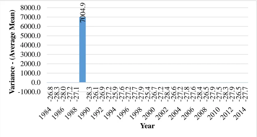
Comparing the annual variance from long term mean temperature of 31 0C, the variation is very high in the year 1989 and low in other years for the time considered-1984-2014, Figure 4.8.

Figure 3: Temperature variability from long term means (1984-2014) Source: KMD (2017).

Comparison between 10-year period shown in Figure 4.9, from 1984 to 1993, the month of March had an average temperature of 600C while July and August were 280C. In 1994 and 2003, the months of February and March recorded the highest temperature of

y = -0.0684x + 32.214 R² = 0.0219

0.0 10.0 20.0 30.0 40.0 50.0 60.0 T em per at ur e (oC ) Year

Temperature (oC) Linear (Temperature (oC))

-26.8 -28.3 -28.0 -27

.2

-27.1

7004.9

(38)

26

330C while the lowest recorded was 280C in July and August. Similar to the period between 1994 and 2003, February recoded 330C while the months of July and August had 280C.

Figure 4: Mean temperature over 10 yr. period Source: KMD (2017).

The ANOVA test in Table 4.7 shows that the temperature between 1984 and 1993 have the highest average temperature of 32 0C and high variance of 85 0C which is higher than variance of 40 C for 1994 to 2003 and 3 0C for 2004 to 2014.

Table 4. 7: ANOVA single factor test summary for temperature SUMMARY

Groups Count Sum Average Variance

1984 to 1993 12 389.84 32.48667 85.29833

1994 to 2003 12 363.41 30.28417 3.809845

2004 to 2014 12 367.6545 30.63788 3.348983

Source: Field Work (2017).

The test of significance shows (Table 4.8) that the sums of squares between the 10-year category is 33 0C and within the category is 1017 0C. The test further reveals that the P-value is 0.58 which is higher than the 0.05 p-P-value for 95% confidence level.

The sum of squares is higher for temperature within the 10-year periods than between the 10 year periods, thus an indication that the temperature within 10-year period has

0.0 20.0 40.0 60.0 80.0

JAN FEB MAR APR MAY JUN JUL AUG SEP OCT NOV DEC

T

em

per

at

ur

e

(o

C)

Month

(39)

27

greater impact on the overall temperature than the temperatures between 10-year periods.

Table 4. 8: ANOVA significance test for temperature

Source of Variation

SS df MS F P-value F crit

Between Groups

33.57654 2 16.78827 0.544737 0.58512 3.284918

Within Groups

1017.029 33 30.81905

Total 1050.605 35

4.2.2 Rainfall

(40)

28 Figure 5: Monthly Rainfall (1986-2014) Average Source: KMD (2017).

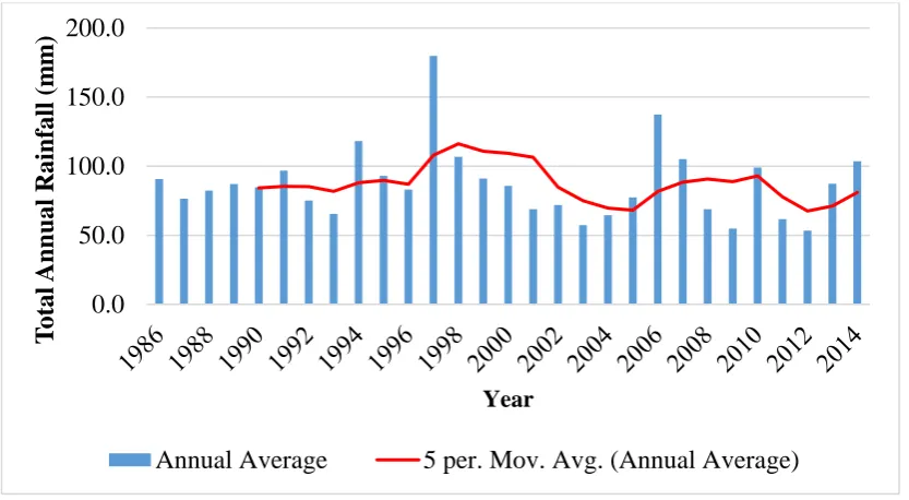
The annual rainfall for Mombasa between 1986 to 2014 (Figure 4.11) showed that the county had highest precipitation (180mm) in 1997 followed by 138mm in 2006. Other years with precipitations above 100mm were 1998 (107mm), 2007 (105) and 2014 (103). The moving average of years through the years showed a high precipitation in 1998 and the lowest in 2012.

Figure 6: Total annual Rainfall (mm) for Mombasa (1986-2014) Source: KMD (2017).

0.0 50.0 100.0 150.0 200.0 250.0 300.0

P

re

cip

ita

tion

(

m

)

Months Precipitation (mm)

0.0 50.0 100.0 150.0 200.0

T

ot

al

A

nn

ual

R

ain

fall

(m

m

)

Year

(41)

29

The rainfall variability from the long term mean of 87mm indicated (Figure 4.11) high positive variability in the year 1997 while the rest of the years have lower variability with the lowest negative variability in 1995 (-29mm) and lowest positive variability in 1987 (422mm).

The data above shows that rainfall pattern has changed over time considering that between 1986 and 1991, Mombasa experienced a steady rainfall about 10mm i.e., between 76 mm to 96 mm. This predictable trend drastically changed from 1992 through 2014. As shown in Figure 4.11, the 5year moving average was highly not predictable with the actual rainfall especially between 1999 and 2003 since there were considerably high difference in the predicted and actual precipitations. From the year 2005 through 2014, the difference in the moving average and actual precipitations increased from ± 10 to ± 20 mm compared to rainfall variation between 1986 to 1991. Thus, an indication that the degree of unpredictability of rainfall precipitations increases over time in Mombasa.

This agrees with the studies by Boko et al., 2007; Bowden and Semazzi, 2007; Funk et al., 2008 which found that there is irregular and shifting rainfall pattern across the coastal areas in Africa.

Figure 7: Rainfall Variability from long term means 987mm) 1986-2014. Source: KMD (2017).

-20000.0 -10000.0 0.0 10000.0 20000.0 30000.0 40000.0 50000.0

1986 1988 1990 1992 1994 1996 1998 2000 2002 2004 2006 2008 2010 2012 2014

V

ar

ian

ce

f

rom

lon

g

te

rm

M

ean

(m

m

)

(42)

30

Comparison between 10 years’ period categories in Figure 4.13 showed that the mean rainfall was lower in the months of February (specifically 6mm for 1986 to1995), January (specifically 10mm for 2006 to 2014), March (36mm 1996 to 2005) and June. Precipitation was high (2695mm) in May within 1986 to 1995, 215mm within 1996 to 2005, and 253mm between 2006 and 2014.

Figure 4.13: Mean rainfall over 10yr. period. Source: KMD (2017).

The ANOVA test in Table 4.9 shows that the rainfall between 1996 and 2005 have the highest average rainfall of 89mm and with a lower variance of 3656 compares to the other 10 years’ period categories.

Table 4. 9: ANOVA single factor test summary for rainfall SUMMARY

Groups Count Sum Average Variance

1986 to 1995 12 7539.36 628.28 561241.3

1996 to 2005 12 1064.048 88.67067 3656.467 2006 to 2014 12 1019.521 84.96007 4889.923 Source: KMD (2017)

The test of significance shows (Table 4.9) that the sums of squares between the 10 years’ categories is 2345554 mm and within categories is 6267664 mm. The test further revealed that the P-value is 0.0052 which is lower than the 0.05 p-value for 95% confidence level.

0.0 100.0 200.0 300.0

0.0 1000.0 2000.0 3000.0

R

ain

fall

(m

m

)

Month

(43)

31

The sum of squares is higher for rainfall within the 10 years’ periods than between the 10 years’ periods, thus an indication that the rainfall within 10 years’ period has greater impact on the overall rainfall than the rainfalls between 10 years’ periods. The F-value indicates the level of difference between the groups than within the groups.

Table 4. 10: ANOVA significance test for rainfall

Source of Variation

SS df MS F P-value F crit

Between Groups

2345554 2 1172777 6.174811 0.005272 3.284918

Within Groups

6267664 33 189929.2

Total 8613219 35

Source: KMD Data (2017).

4.3 Effect of Sea Level Rise on Communities in Study Area for Past 30 Year. Sea level raise can cause flood which ultimately have financial effects. However, there are positive and beneficial effect of salt water made available from the raise in sea level. 4.3.1 Effects of Flood on Income

(44)

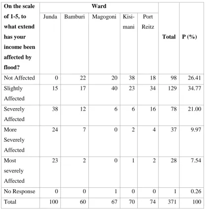
32 Table 4. 11: Flood effect on respondents' income.

On the scale of 1-5, to what extend has your income been affected by flood?

Ward

Total P (%) Junda Bamburi Magogoni

Kisi-mani

Port Reitz

Not Affected 0 22 20 38 18 98 26.41

Slightly Affected

15 17 40 23 34 129 34.77

Severely Affected

38 12 6 6 16 78 21.00

More Severely Affected

24 7 0 2 4 37 9.97

Most severely Affected

23 2 0 1 2 28 7.54

No Response 0 0 1 0 0 1 0.26

Total 100 60 67 70 74 371 100

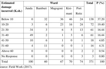
4.3.2 Estimated Damage of Flood

(45)

33

there is an increasing rise in the damages caused by flood and one of the reasons is the increase in precipitation.

Table 4. 12: Respondents' estimated damage caused by flood Estimated

damage

incurred (K.sh.)

Ward Total P (%)

Port Reitz

Below 10 0 32 36 46 24 138 37.20

10-20 3 6 23 16 24 72 19.40

21-30 34 3 6 5 13 61 16.44

31-40 49 2 1 3 6 61 16.44

41-50 10 6 1 0 1 18 4.85

51-60 4 11 0 0 1 16 4.31

Above 60 0 0 0 0 2 2 0.54

No Response 0 0 0 0 3 3 0.80

Total 100 60 67 70 74 371 100

4.3.3 Occurrence of similar-flood causing damages

Majority of the respondents 93% stated that similar flooding that cost them an estimated damage usually occurs annually (Table 4.13). Thus, an indication that on average, each of the respondents loses an estimated amount of 10,000 to 20,000 Kenyan shillings annually.

Table 4. 13: Respondents' frequency estimated damage caused by flood. When do you

expect similar flooding

Ward Total Perce

nt (%) Junda Bamburi Magogoni Kisi

man

Port Reitz

Every Yrs. 88 57 67 60 74 346 93.26

Every 2 Yrs. 11 1 0 9 0 21 5.66

Every 8 Yrs. 0 2 0 0 0 2 0.53

No response 1 0 0 1 0 2 0.53

Total 100 60 67 70 74 371 100

(46)

34 4.3.4 Benefit of Fresh and Salt water

The majority (55%) of the respondents as shown in Table 4.14 indicated that they benefit from fresh and salt water flooding most of which are little benefits (43%). Within the wards: majority of the respondents in Magogoni, Kisimani and Port Reitz do not benefit from the salt/salt water.

Table 4. 14: Respondents' benefit from fresh and salt water floods. What benefit

do you get from flooding

Ward

Total P(%) Junda Bamburi Magogoni

Kisi-mani

Port Reitz

No Benefit 33 22 29 42 40 166 44.74

Little Benefit 38 30 37 25 30 160 43.13

More Benefit 20 8 1 3 4 36 9.70

Most Benefit 9 0 0 0 0 9 2.43

Total 100 60 67 70 74 371 100.00

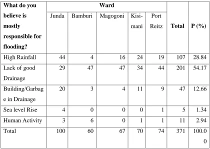
4.3.5 Perception on the Causes of Flooding

The respondents’ majority (54%) as shown in Table 4.15 believes that lack of good drainage system is the cause of flooding. Other perceptions include high rainfall (29%), construction of buildings and garbage obstruction of drainages (13%), human activities (3%) and rise of sea level (1%). Within the wards: high rainfall (44%) was responsible for flooding in Junda.

(47)

35 Table 4. 15: Respondents' perception on flooding

What do you believe is mostly

responsible for flooding?

Ward

Total P (%) Junda Bamburi Magogoni

Kisi-mani

Port Reitz

High Rainfall 44 4 16 24 19 107 28.84

Lack of good Drainage

29 47 47 34 44 201 54.17

Building/Garbag e in Drainage

20 3 4 11 9 47 12.66

Sea level Rise 4 0 0 0 1 5 1.34

Human Activity 3 6 0 1 1 11 2.94

Total 100 60 67 70 74 371 100.0

0

Source: Field Work (2017). 4.3.6 Frequency of Flood

(48)

36 Table 4. 16: frequency of flooding

How frequent does flooding occur here?

Ward Total P (%)

Port Reitz

Once/Yr. 90 59 52 64 51 316 85.17

Once/2Yrs 9 1 0 6 0 16 4.31

Twice/Yrs 0 0 14 0 23 37 9.97

No Response 1 0 1 0 0 2 0.54

Total 100 60 67 70 74 371 100.00

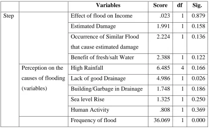
4.3.7 Hypothesis Testing for Effect of Sea-level Rise Variables

Using Binary Logistics Regression (BLR): The H1 (alternative hypothesis), i.e., Sea Level Rise significantly influence the indigenous means to mitigate and adapt to flooding and climate variability impact is accepted because the P-value is less than 0.05 as shown in the Table 4.17

Table 4. 17: Dependent variable for sea level rise hypothesis Variables in the Equation

B S.E. Wald Df Sig. Exp-B Step Constant -1.836 0.151 148.363 1 0.000 0.159

The Binary Logistics Regressions (BLR) model for the Sea Level Rise BLR equation is:

1 1 ) 836 . 1 ( ) 1

ln( B X

p

p ₌ ₋ ₊

−

(49)

37

Table 4. 18: sea level rise variables not in the equation

Variables Score df Sig.

Step Effect of flood on Income .023 1 0.879 Estimated Damage 1.991 1 0.158 Occurrence of Similar Flood

that cause estimated damage

2.224 1 0.136

Benefit of fresh/salt Water 2.388 1 0.122 Perception on the

causes of flooding (variables)

High Rainfall 6.485 4 0.166

Lack of good Drainage 4.986 1 0.026 Building/Garbage in Drainage 1.748 1 0.186 Sea level Rise 1.325 1 0.250

Human Activity .808 1 0.369

Frequency of flood 36.069 1 0.000

Based on the hypothesis rule, at least one of the independent variable must be statistically significant to accept Hi. As shown above, at least one of the sea level rise variables are statistically significant in step 1, thus H1 for sea level rise is accepted. Table 4. 19: Sea level rise variable in the equation

B S.E. Wald df Sig. Exp(B) Step

1a

Lack of good Drainage

-.734 1.021 .517 1 .472 .480

Frequency of flood .395 .079 25.240 1 .000 1.484

Constant 15.55

0

4849.3 89

.000 1 .997 5664471. 912 a. Variable(s) entered on step 1: Only statistically significant sea level rise variables from step 0.

(50)

38

Since the constant for sea level rise is 15.550, the SLR equation model for the sea level rise is

) ( ) 550 . 15 ( ) 1

ln( B1iX1i

p

p ₌ ₊

−

Where,

(51)

39

4.4 Role of Environmental Education on Flood Impact Adaptation and Mitigation as Results of Sea Level Rise.

For there to be mitigation of flooding due to sea level rise, its impact and adaptability to the un-prevented floods, there is need for environmental education with specific emphasis on the knowledge about flood predictions, the reliability and challenges of such predictions.

4.4.1 Knowledge on Flood Prediction

The majority (34%) of respondent stated that media in form of television and radio are the means through which they are informed on the possibility of flood occurrence (Table 4.20). Other means includes their personal experience (26%), Barazza (17%), their personal observation (12%), and KMD (11%). This is an indication that their personal prediction through observation and experience (38%) is the chief means through which the respondents predicts the likelihood of flooding.

Within the respective wards: Junda is heavily (41%) reliant on Barazza as flood prediction information source; Bamburi and Kisimani are chiefly through personal experience and observation; while Magogoni and Port Reitz are through the Media. This agrees with Adebayo et al., (2011) that basic observation and experience of rural settlers increases their knowledge about flooding. However, the increasing portability of media devices and accessibility of those devices to life-helping information is increasing due to digital flow of information as rightly referred by James (2012).

Table 4. 20: Respondents' prediction on the occurrence of flood How do

you know when it will flood?

Ward

Total P (%) Junda Bamburi Magogoni Kisimani Port

Reitz

Experience 12 20 15 27 21 95 25.60

Observation 8 6 7 17 7 45 12.12

KMD 17 10 3 8 4 42 11.32

Barazza 41 11 1 7 2 62 16.71

Media (Radio/TV)

22 13 41 11 40 127 34.23

Total 100 60 67 70 74 371 100.00

(52)

40 4.4.2 Reliability of the Knowledge

Out of the 371 respondents (Table 4.21): majority 38% stated that their predictions about the occurrence of flood is less reliable; 27% stated more reliable; 18% not reliable; and 16% most reliable. Within the respective wards: 46% stated most reliable in Junda; 35% stated more reliable in Bamburi; 55% stated less reliable in Magogoni; 43% stated not reliable in Kisimani; and 59% stated less reliable in Port Reitz.

This indicates that their source of information chiefly through personal experience and observation is not or is less reliable (56%). The precipitation changes and irregular rainfall pattern as revealed by the Data from KMD may have accounted for the less reliability. This finding agrees with (Slovic, Fischhoff, and Lichtenstein, 1979) in his findings that memorable past flood events is chiefly the factor an individual use to predict flood occurrence, but this prediction is only to the extent and magnitudes of floods they had earlier experienced and thus with the irregular rainfall pattern as reveled by KMD data, the respondents’ prediction may be unreliable as they face more often new or different flood experience.

Table 4. 21: Reliability of respondents' prediction on the occurrence of flood How reliable is

your prediction

Ward Total P (%)

Port Reitz

Not Reliable 1 18 10 30 8 67 18.05

Less Reliable 16 18 37 26 44 141 38.00

More Reliable 37 21 15 11 18 102 27.49

Most Reliable 46 3 5 3 4 61 16.44

Total 100 60 67 70 74 371 100.00

4.4.3 Challenges to Good Flood Prediction

(53)

41

deforestation, fishing and animal grazing are the major challenges to good prediction of flood, rainfall, and drought. Within the respective wards: sand mining is the major (73%) hindrance in Junda; while deforestation is of concern in Bamburi (67%), Magogoni (84%), Kisimani (57%), and Port Reitz (77%). The respondents (87%) identified anthropogenic activities that have caused the low reliability on their knowledge about the occurrence of flood, rainfall and drought. Those activities changes render actual predations to be false since those activities potentially alter the environmental conditions and its usual patterns. This confirms Salick & Byg, (2007:11) findings that there is reduction in the preciseness of flood prediction by the community due to vulnerability to climate change.

Table 4. 22: Challenges to respondents' prediction on the occurrence of flood Which

activity interferes with your ability to know when flooding, rainfall or drought will occur

Ward Total P (%)

Port Reitz

Farming /deforestation

13 40 56 40 57 206 55.52

Fishing 3 8 5 26 7 49 13.20

Animal Grazing

6 1 0 1 3 11 2.96

Sand Mining 73 11 6 1 1 92 24.80

No Response 5 0 0 2 6 13 3.50

Total 100 60 67 70 74 371 100.0

0

4.4.4 Distance of Respondents’ Livelihood from River-bank/Seashore

(54)

42

22% indicated a distance above 2001 metres; 20% between 1001 to 1500 metres; 17% between 1501 to 2000 meters; and 11% between 501 to 1000 meters. Within the wards: majority (98%) in Junda stated a distance below 500 meters; 47% in Bamburi between stated above 2001 metres; 36% in Magogoni between 1501 to 2000 meters; 50% in Kisimani between 1001 to 1500 metres; and 47% in Port Reitz between 501 to 1000 metres.

Majority of the respondents especially those in Junda are highly prone to flooding caused by overflow of riverbank because they live close to the riverbank.

Table 4. 23: Respondents' activity distance from Riverbank and Seashore How far

away from the seashore /river bank is your farm, business, Housing or approx. in meters (m)

Ward

Total P (%) Junda Bamburi Magogoni

Kisi-mani

Port Reitz

Below 500 m 98 1 1 1 6 107 28.84

501-1000 m 2 2 2 4 35 45 11.05

1001-1500 m 0 18 18 35 3 74 19.95

1501-2000 m 0 11 24 13 17 65 17.52

Above 2001 m

0 28 22 17 13 80 21.56