Scholarship@Western
Scholarship@Western
Electronic Thesis and Dissertation Repository
8-6-2019 2:00 PM
Advances in Moment-Based Distributional Methodologies
Advances in Moment-Based Distributional Methodologies
Yishan Zang
The University of Western Ontario
Supervisor Provost, Serge B.
The University of Western Ontario
Graduate Program in Statistics and Actuarial Sciences
A thesis submitted in partial fulfillment of the requirements for the degree in Master of Science © Yishan Zang 2019
Follow this and additional works at: https://ir.lib.uwo.ca/etd
Part of the Statistical Methodology Commons
Recommended Citation Recommended Citation
Zang, Yishan, "Advances in Moment-Based Distributional Methodologies" (2019). Electronic Thesis and Dissertation Repository. 6304.
https://ir.lib.uwo.ca/etd/6304
This Dissertation/Thesis is brought to you for free and open access by Scholarship@Western. It has been accepted for inclusion in Electronic Thesis and Dissertation Repository by an authorized administrator of
This thesis includes various results that rely on the moments of a distribution or the sample
moments associated with a set of observations. Since a sample of sizenis uniquely specified by
its firstnmoments, it is pertinent to make use of sample moments for modeling, classification
or statistical inference purposes. Three density mixtures are approximated by adjusting in
various ways an initial density approximation referred to a base density by means of certain
moment-based functions, and the accuracy of the resulting density approximants are compared.
A similar study is carried out in the context of density estimation. Moreover, it is explained
that methodologies that are based on moments are, in fact, ideally suited to model massive
data sets. Various types of quasi-Monte Carlo deterministic samples are then compared to
randomly generated samples with respect to their distributional representativeness. As well,
a novel methodology depending on an arctangent transformation is introduced for classifying
the tail behaviour of probability laws. Finally, certain approximations to the distributions of
quadratic forms in gamma, inverse Gaussian, binomial and Poisson random variables, which
rely on a symbolic expansion of their moments, are proposed.
Keywords: Density approximation, data modeling, quasi-Monte Carlo samples, classification
of tail behaviour, quadratic forms.
Various statistical results of interest that are based on the moments of a distribution are
presented in this thesis. In fact, the moments associated with a sample of observations contain
all the distributional information therein available. Several types of adjustments and samples
are investigated in order to determine which ones will provide the most accurate
representa-tions of a given distribution. As well, a simple new criterion is proposed to categorize the tail
behaviour of probability laws. Finally, an efficient approach is proposed for approximating
the distribution of quadratic forms in several types of random variables, which are utilized in
connection with contingency tables and generalized linear models.
First of all, I am very grateful to my supervisor, Professor Serge B. Provost, for his
dedi-cated and inspiring guidance, which greatly improved my research and writing skills. Thanks
are also due to the thesis examiners, Neil Klar, Wenqing He and Jiandong Ren. I would also like
to express my sincere thanks to the Department of Statistical and Actuarial Sciences and the
School of Graduate and Postdoctoral Studies for their financial support. Finally, I am indebted
to my parents for their love, encouragement and support.
Abstract ii
Summary iii
Dedication iv
Acknowledgements v
List of Figures ix
List of Tables xvi
List of Appendices xvii
1 Introduction 1
2 On Comparing Various Types of Moment-Based Density Approximants 9
2.1 Introduction . . . 9
2.2 Seven types of moment-based density approximants . . . 10
2.2.1 Approximants expressed as the product of a base density and a
polyno-mial (Type 1) . . . 10
2.2.2 Approximants expressed as polynomials (Type 2) . . . 12
2.2.3 Approximants expressed as the sum of a base density and a polynomial
(Type 3) . . . 13
nentiated polynomial (Type 4) . . . 15
2.2.5 Differentiated logdensity approximants (DLA) (Type 5) . . . 16
2.2.6 Approximants expressed in terms of a base density and a DLA (Type 6) 17 2.2.7 Approximants expressed as a mixture of a base density and a DLA (Type 7) . . . 18
2.3 Obtaining a bona fide density function . . . 19
2.4 Application of the methodologies . . . 19
2.4.1 Mixture of beta pdf’s . . . 19
2.4.2 Mixture of gamma pdf’s . . . 22
2.4.3 Mixture of normal pdf’s . . . 26
3 On Comparing Various Types of Moment-Based Density Estimates 31 3.1 Introduction . . . 31
3.2 Simulated data . . . 32
3.2.1 A mixture of beta pdf’s . . . 32
3.2.2 A mixture of gamma pdf’s . . . 35
3.3 Examples . . . 38
3.3.1 The Buffalo snowfall data . . . 38
3.3.2 The Old Faithful geyser data . . . 41
3.3.3 A large data set: US household income in 2016 . . . 44
4 Certain Types of Samples and their Distributional Representativeness 48 4.1 Introduction . . . 48
4.2 Types of samples and criteria for determining their distributional representa-tiveness . . . 49
4.3 Assessment of distributional representativeness . . . 50
4.3.1 Sample generated from a beta(2,5) distribution . . . 50
5 A New Methodology for Characterizing Distributional Tail Behaviour 59
5.1 Introduction . . . 59
5.2 Classifying the right tail of a distribution by means of the arctan transformation 61 5.3 Comparison with other criteria . . . 63
6 Quadratic Forms in Various Types of Random Variables 68 6.1 Introduction . . . 68
6.2 On evaluating the exact moments of quadratic forms via the symbolic approach 69 6.3 Applications . . . 71
6.3.1 Quadratic forms in gamma random variables . . . 71
6.3.2 Quadratic forms in inverse Gaussian random variables . . . 75
6.3.3 Quadratic forms in binomial random variables . . . 78
6.3.4 Quadratic forms in Poisson random variables . . . 81
7 Concluding Remarks and Future Work 86
Appendix A Mathematica Code 88
Curriculum Vitae 141
2.1 Exact PDF and base density . . . 20
2.2 f1,n=10 . . . 20
2.3 f2,n=10 . . . 20
2.4 f3,n=10 . . . 20
2.5 f4,n=10 . . . 20
2.6 f4,n=13, best approximation . . . 20
2.7 f5,ν=11,δ=0 . . . 21
2.8 f5,ν=17,δ=0, best approximation . . . 21
2.9 f6,ν=9 . . . 21
2.10 f6,ν=12,δ=0, best approximation . . . 21
2.11 f7,w=0.3,ν=7,δ =0 . . . 21
2.12 f7,w=0.2,ν=15,δ =0 . . . 21
2.13 Exact density . . . 23
2.14 Transformed PDF’s . . . 23
2.15 f1,n=10 . . . 23
2.16 f1,n=25, best approximation . . . 23
2.17 f2,n=10 . . . 23
2.18 f2,n=12, best approximation . . . 23
2.19 f3,n=10 . . . 23
2.20 f3,n=12, best approximation . . . 23
2.21 f5,ν=10,δ=0 . . . 24
2.23 f7,w=0.1,ν=13,δ =0 . . . 24
2.24 f7,w=0.2,ν=11,δ =0 . . . 24
2.25 Truncated distribution . . . 25
2.26 Exact PDF and base density . . . 25
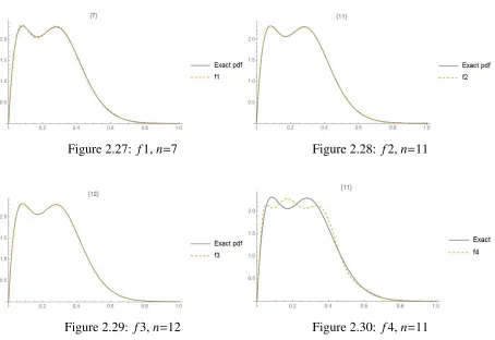
2.27 f1,n=7 . . . 25
2.28 f2,n=11 . . . 25
2.29 f3,n=12 . . . 25
2.30 f4,n=11 . . . 25
2.31 f5,ν=17,δ=0 . . . 26
2.32 f7,ν=21,δ=0 . . . 26
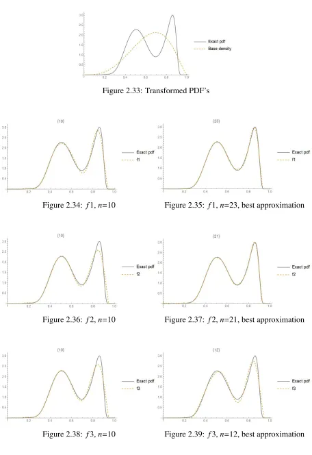
2.33 Transformed PDF’s . . . 27
2.34 f1,n=10 . . . 27
2.35 f1,n=23, best approximation . . . 27
2.36 f2,n=10 . . . 27
2.37 f2,n=21, best approximation . . . 27
2.38 f3,n=10 . . . 27
2.39 f3,n=12, best approximation . . . 27
2.40 f5,ν=9,δ=0 . . . 28
2.41 f5,n=16,δ =0, best approximation . . . 28
2.42 f7,w=0.1,ν=11,δ =0 . . . 28
2.43 Mixture distribution PDF and base PDF . . . 29
2.44 f1,n=40 . . . 29
2.45 f1,n=60 . . . 29
2.46 f1,n=90 . . . 29
3.1 Mixture of beta PDF’s . . . 33
3.2 Histogram and kernel density . . . 33
3.4 Empirical CDF and kernel CDF, (SSD=0.0832852) . . . 33
3.5 Histogram, kernel density and f1 . . . 33
3.6 Empirical CDF andF1 . . . 33
3.7 Histogram, kernel density and f2 . . . 33
3.8 Empirical CDF andF2 . . . 33
3.9 Histogram, kernel density and f3 . . . 34
3.10 Empirical CDF andF3 . . . 34
3.11 Histogram, kernel density and f5 . . . 34
3.12 Empirical CDF andF5 . . . 34
3.13 Histogram, kernel density and f7,w= 0.1 . . . 34
3.14 Empirical CDF andF7,w=0.1 . . . 34
3.15 Mixture of gamma PDF’s . . . 35
3.16 Histogram and kernel density . . . 35
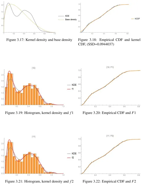
3.17 Kernel density and base density . . . 36
3.18 Empirical CDF and kernel CDF, (SSD=0.0944037) . . . 36
3.19 Histogram, kernel density and f1 . . . 36
3.20 Empirical CDF andF1 . . . 36
3.21 Histogram, kernel density and f2 . . . 36
3.22 Empirical CDF andF2 . . . 36
3.23 Histogram, kernel density and f3 . . . 37
3.24 Empirical CDF andF3 . . . 37
3.25 Histogram, kernel density and f5 . . . 37
3.26 Empirical CDF andF5 . . . 37
3.27 Histogram, kernel density and f7,w= 0.1 . . . 37
3.28 Empirical CDF andF7,w=0.1 . . . 37
3.29 Histogram of the Buffalo snowfall data . . . 39
3.31 Empirical CDF and kernel CDF, (SSD=0.0286895) . . . 39
3.32 kde (grey line) and f1,n=10 . . . 39
3.33 ECDF andF1,n=10 . . . 39
3.34 kde (grey line) and f2,n=11 . . . 40
3.35 ECDF andF2,n=11 . . . 40
3.36 kde (grey line) and f3,n=11 . . . 40
3.37 ECDF andF3,n=11 . . . 40
3.38 kde (grey line) and f5,ν=6,δ=0 . . . 40
3.39 ECDF andF5,ν=6,δ =0 . . . 40
3.40 kde (grey line) and f7,ν=6,δ=0 . . . 41
3.41 ECDF andF7,ν=6,δ =0 . . . 41
3.42 Histogram of the Old Faithful data . . . 42
3.43 kde (grey line) and base density . . . 42
3.44 Empirical CDF and kernel CDF, (SSD=0.257145) . . . 42
3.45 kde (grey line) and f1, n=12 . . . 42
3.46 ECDF andF1, n=12 . . . 42
3.47 kde (grey line) and f2,n=9 . . . 43
3.48 ECDF andF2,n=9 . . . 43
3.49 kde (grey line) and f3,n=10 . . . 43
3.50 ECDF andF3,n=10 . . . 43
3.51 kde (grey line) and f5,n=7,δ=0 . . . 43
3.52 ECDF andF5,ν=7,δ=0 . . . 43
3.53 Histogram of the US household income data . . . 44
3.54 kde (grey line) and base density . . . 45
3.55 Empirical CDF and kernel CDF, (SSD=0.0923982) . . . 45
3.56 kde (grey line) and f1,n=19 . . . 45
3.58 kde (grey line) and f2,n=20 . . . 45
3.59 ECDF andF2,n=20 . . . 45
3.60 kde (grey line) and f3,n=12 . . . 46
3.61 ECDF andF3,n=12 . . . 46
3.62 kde (grey line) and f5,ν=5,δ=0 . . . 46
3.63 ECDF andF5,ν=5,δ =0 . . . 46
3.64 kde (grey line) and f7,w=0.1,ν=5,δ =0 . . . 46
3.65 ECDF andF7,w=0.1,ν=5,δ= 0 . . . 46
4.1 Beta(2,5) PDF . . . 51
4.2 Samples of 5 types . . . 51
4.3 kde’s for types 1 & 2 samples (left panel) and types 3, 4 & 5 samples (right panel) 51 4.4 Exact and empirical CDF’s for the 5 types of samples . . . 52
4.5 Corrected ECDF’s for the 5 types of samples . . . 52
4.6 PDF of the mixture . . . 54
4.7 Samples of 5 types . . . 54
4.8 kde’s for types 1 & 2 samples (left panel) and types 3, 4 & 5 samples (right panel) 54 4.9 Exact and empirical CDF’s for the 5 types of samples . . . 55
4.10 Corrected ECDF’s for the 5 types of samples . . . 55
5.1 Normal distribution, fz(z) . . . 63
5.2 Weibull distribution (k=2), fz(z) . . . 63
5.3 Extreme value distribution, fz(z) . . . 63
5.4 Logistic distribution, fz(z) . . . 63
5.5 Exponential distribution, fz(z) . . . 64
5.6 t-distribution,ν= 3 fz(z) . . . 64
5.7 Lognormal(0, 1) distribution, fz(z) . . . 64
6.1 PDF’s ofX1andX2 . . . 72
6.2 Histogram and the base density . . . 73
6.3 Empirical CDF and the base CDF . . . 73
6.4 Histogram and f1 . . . 73
6.5 Empirical CDF and F1 . . . 73
6.6 PDF’s ofXi’s . . . 74
6.7 Histogram and the base density ofY . . . 74
6.8 Empirical CDF and the base CDF . . . 74
6.9 Histogram and f1 . . . 74
6.10 Empirical CDF andF1 . . . 74
6.11 PDF’s ofX1andX2 . . . 75
6.12 Histogram and the base density ofY . . . 75
6.13 Empirical CDF and the base CDF . . . 75
6.14 Histogram and f1 . . . 76
6.15 Empirical CDF andF1 . . . 76
6.16 PDF’s ofXi’s . . . 76
6.17 Histogram and the base density ofY . . . 77
6.18 Empirical CDF and the base CDF . . . 77
6.19 Histogram and f1 . . . 77
6.20 Empirical CDF andF1 . . . 77
6.21 CDF’s ofX1andX2 . . . 78
6.22 Histogram and the base density ofY . . . 79
6.23 Empirical CDF and the base CDF . . . 79
6.24 Histogram and f1 . . . 79
6.25 Empirical CDF andF1 . . . 79
6.26 CDF’s ofXi’s . . . 80
6.28 Empirical CDF and the base CDF . . . 80
6.29 Histogram and f1 . . . 80
6.30 Empirical CDF andF1 . . . 80
6.31 CDF’s ofX1andX2 . . . 81
6.32 Histogram and the base density ofY . . . 82
6.33 Empirical CDF and the base CDF . . . 82
6.34 Histogram and f1 . . . 82
6.35 Empirical CDF andF1 . . . 82
6.36 CDF’s ofXi’s . . . 83
6.37 Histogram and the base density ofY . . . 83
6.38 Empirical CDF and the base CDF . . . 83
6.39 Histogram and f1 . . . 83
6.40 Empirical CDF andF1 . . . 83
2.1 Comparison of the ISD’s for different types and degrees . . . 22
2.2 Comparison of the ISD’s for different types and degrees . . . 24
2.3 Comparison of the ISD’s for different types and degrees . . . 26
2.4 Comparison of the ISD’s for different types and degrees . . . 28
2.5 Comparison of the ISD’s for different degrees (Type 1 approximant) . . . 29
3.1 Optimal density estimates of various types and SSD’s . . . 35
3.2 Optimal density estimates of various types and SSD’s . . . 38
3.3 Optimal density estimates of various types and SSD’s . . . 41
3.4 Optimal density estimates of various types and SSD’s . . . 44
4.1 Relative errors between sample and exact moments . . . 53
4.2 Rankings of the criteria for determine the most representative samples . . . 53
4.3 Average of the criteria values . . . 53
4.4 Relative errors between sample and exact moments . . . 56
4.5 Rankings of criteria for determining the most representative samples . . . 56
4.6 Average of the criteria values . . . 56
5.1 Tail behavior classification for certain distributions . . . 61
5.2 Classification of tail behaviour . . . 62
5.3 Comparative classification of tail behavior for certain distributions . . . 65
5.4 Classification of the tail behavior of some other distributions . . . 66
Appendix A Mathematica code . . . 88
Introduction
Several distribution approximation techniques that rely on the moments or the cumulants of a
random variable have been proposed in the statistical literature. For example, approximants
of this type can be obtained by making use of Pearson or Johnson curves, see Solomon and
Stephens (1978), Elderton and Johnson (1969) and Rose and Smith (2002), or saddlepoint
approximations as discussed in Reid (1988). These methodologies can provide adequate
ap-proximations in a variety of applications involving unimodal distributions. However, they may
prove difficult to implement. The approximants proposed in this thesis have relatively simple
functional forms that lend themselves to algebraic manipulations and apply to a very wide
ar-ray of distributions. Moreover, their accuracy can be improved by making use of additional
moments. Interestingly, another technique called the inverse Mellin transform, which is based
on the complex moments of certain distributions, provides representations of their exact
den-sity functions in terms of generalized hypergeometric functions; for theoretical considerations
as well as various applications, the reader is referred to Mathai and Saxena (1978) and Provost
and Rudiuk (1995).
There exist several types of density estimates and approximants. However, many of these
techniques will fail to provide adequate approximations, especially when the target density is
not a smooth unimodal function. Silverman (1986) provides a survey of the various available
methodologies. Efromovich (1999) presents a unified account of nonparametric approaches
to density estimation. Other types of nonparametric density estimates that are based on the
L1norm are presented in Devroye (1985) while both parametric and nonparametric approaches
are discussed in Eggermont (2001). The multivariate case is extensively treated in Scott (2015).
Two of the main approaches advocated in Chapter 2 are based on Results 1 and 2. First,
the exact density function associated with a distribution whose first n moments are known
can be approximated by means of the product of a base density function, whose parameters
are determined by matching moments, and a polynomial of degreen, whose coefficients are
obtained by making use of the method of moments. This general semiparametric approach to
density approximation, which appeared in Provost (2005), is formally stated in the following
result.
Result 1 Let fY(y)be the density function of a continuous random variable Y defined in the
interval(a,b), E(Yj)≡µY(j), X =(Y −u)/s be an affine transformation (oftentimes, u= E(Y)
and s= √Var(Y)), where u∈IRand s ∈IR+, a0= (a−u)/s, b0 =(b−u)/s, fX(x)= s fY(u+s x)
denote the density function of X whose support is the interval(a0,b0), E(Xj)= E[((Y−u)/s)j]≡
µX(j), and let the base density function ψX(x) ≡ cTw(x), where cT is a positive normalizing
constant, be an initial density approximation to fX(x)with
Rb0 a0 x
jψX
(x) dx ≡ mX(j).Assuming
that the sequenceµX(i), i= 0,1,2, . . . ,uniquely defines the distribution of X, that mX(j)exists
for j = 0,1, . . . ,2n, and that wheneverψX(x) is nontrivial function of x, its tail behavior is
congruent to that of fX(x), the density function of X can be approximated by
fXn(x)=ψX(x) n
X
`=0
ξ`x` (1.1)
with(ξ0, . . . , ξn) 0
= M−1(µX(0), . . . , µX(n))0, where M is an(n+1)×(n+1)matrix whose(h+1)th
row is mX(h), . . . ,mX(h+n), h = 0,1, . . . ,n. WhenψX(x)depends on r parameters, these are
determined by equating mX(j)to µX(j), j = 1, . . . ,r. The corresponding density approximant
fYn(y)=ψX
y−u s
Xn
`=0
ξ` s
y−u s
`
. (1.2)
Note that the base density is selected by applying some goodness-of-fit tests, such as the
Kolmogorov-Smirnov and chi-square tests to certain density functions suggested by a
his-togram of the data or the exact density when it is known.
The other primary technique which is summarized in Result 2 yields what is referred to as
differentiated logdensity approximants (DLA’s):
Result 2 Let
fν,δ(x)=k e
Rx
α pν,δ(y) dy (1.3)
be the approximation of a density function defined on the interval(α, β)where
pν,δ(x)=
Pv
i=0aixi
Pδ
j=0cjxj
≡ N(x)
D(x), (1.4)
with cδ=1, k being a positive constant such that fν,δ(·)integrates to one over the interval(α, β).
The function pν,δ(x)is a rational function of ordersνandδand the resulting approximation, as
a differentiated logdensity approximant or DLA.
As shown below, the coefficients ai, i = 0,1, . . . ,v, and cj, j = 0,1, . . . , δ− 1, can be
determined by solving a system of linear equations. On differentiating ln(fν,δ(x)), one obtains
d
dxln(fν,δ(x))= fν,δ0 (x)
fν,δ(x) = pν,δ(x), (1.5)
which yields the relationship,
fν,δ0 (x) δ
X
j=0
cjxj = fν,δ(x)
ν
X
i=0
Then, on multiplying both sides of this equality by xhand integrating fromαtoβ, one has
Z β
α
fν,δ0 (x) δ
X
j=0
cjxj+hdx=
Z β
α
fν,δ(x) ν
X
i=0
aixi+hdx, h=0,1, . . . , ν+δ, (1.7)
which, on integrating the left-hand side by parts, yields
fν,δ(x) δ
X
j=0 cjx
j+h β α− δ X
j=0
cj(j+h)
Z β
α x
j+h−1
fν,δ(x) dx
= ν
X
i=0 ai
Z β
α
xi+hfν,δ(x) dx, h=0,1, . . . , ν+δ,
(1.8)
where
fν,δ(x) δ
X
j=0 cjxj+h
β α = δ X
j=0
cj(fν,δ(β)βj+h− fν,δ(α)αj+h). (1.9)
Thus, lettingµh,h= 0,1, . . . , ν+δ, denote thehth moment of the approximate distribution
specified by fν,δ(x), one has
δ
X
j=0
cj(fν,δ(β)βj+h− fν,δ(α)αj+h−(j+h)µj+h−1)=
ν
X
i=0
ai µi+h, (1.10)
forh= 0,1, . . . , δ+ν, withµ0 = 1. Now, on replacing fν,δ(α), fν,δ(β) andµhby f(α), f(β) and
µX(h),h= 0,1, . . . , δ+ν, respectively, one obtains the recursive relationship,
δ
X
j=0
cj(f(β)βj+h− f(α)αj+h−(j+h)µX(j+h−1))=
ν
X
i=0
ai µX(i+h), (1.11)
forh= 0,1, . . . , δ+ν.
The coefficientsci,i = 0,1, . . . , δ−1, andai,i = 0,1, . . . , ν, can be determined by solving
theseν+δ +1 linear equations. Note that when jand hare both equal to zero, the value of
µX(−1) is not required since its coefficient happens to be zero.
The number of moments that are required for given values of ν and δ can be determined
whereas 2δ+ν+1 moments are required whenδ > ν.
Once the coefficients have been determined, the differential equation,
fν,δ0 (x)= pν,δ(x)fν,δ(x), (1.12)
can be solved by making use of symbolic computational packages such as Mathematica or
Maple. The resulting density approximant is denoted DLA(ν, δ).
This thesis is mainly concerned with methodologies that rely on moments. This is
justi-fied by Result 3 relating a sample to its moments, which was established in Zareamoghaddam
(2018). There are instances in multivariate statistical analysis where the exact distribution of
a test statistic is unknown whereas its exact moments can be determined. Thus the proposed
methodologies are not only useful for modeling purpose but also for making statistical
infer-ence.
Result 3 A set of n observations is uniquely determined by the first n associated sample
mo-ments.
Proof Let S = {x1,x2, . . . ,xn}, M = {m1,m2, . . . ,mn} andmh = Pni=1x
h
i/n. According to the
fundamental theorem of algebra, p(z)=a0+a1z+· · ·+an−1zn−1+znis uniquely specified by
itsnrootsxi’s fori=1,2, . . . ,n.
Moreover, given S, the coefficients of p(x) can be expressed in terms of the sequence of
momentsMvia the Newton-Girard identity. Accordingly, a given polynomial of degreen, say
p(x), can be represented as follows:
n
Y
i=1
(x−xi)= n
X
k=0
(−1)n−ken−kxk, (1.13)
wheree0 =1 and
e` = n` `
X
j=1
(−1)j−1e`−jmj, ` =1, . . . ,n. (1.14)
the right hand side of Equation 1.13, whose roots are precisely x1,x2, ...,xn. This establishes
thatS is uniquely specified byM.
We note that moment-based density estimation techniques are ideally suited for modeling
massive data sets: Once the moments have been evaluated, which is easily achieved even for
extremely large data sets, the determination of the estimated density function does not depend
on the sample size. Moreover, once a new set of observations,Xn1+1, . . . ,Xn, becomes available
in addition to an initial data set, X1, . . . ,Xn1, there is no need to make use of each of the n1
original data points since thehthupdated moment will then be
(n1mh+ n
X
i=n1+1
xhi)/n
wheremhdenotes thehth sample moment evaluated from the initial data set.
Chapter 2 and 3 propose several types of moment-based density approximants and
esti-mates, respectively. In Chapter 4, Monte Carlo samples are compared to quasi-Monte Carlo
samples with respect to their distributional representativeness. An easy-to-apply methodology
is proposed in Chapter 5 for classifying the tail behavior of probability laws. An
approxima-tion to the distribuapproxima-tion of quadratic forms in various types of discrete and continuous random
variables, which is based on a symbolic expansion of their associated moments, is provided in
Chapter 6. Some concluding remarks and an outline of further possible developments in the
area are included in the last chapter. As much effort has been expended on creating the code for
implementing the results presented in this thesis, it is included in the Appendix for the benefit
[1] Devroye, L. and Gyorfi, L. (1985).Nonparametric Density Estimation: The L1View. John
Wiley & Sons, New York.
[2] Efromovich, S. (1999).Nonparametric Curve Estimation: Methods, Theory and
Applica-tions. Springer Science & Business Media, New York.
[3] Eggermont, P. P. B., and LaRiccia, V. N. (2001).Maximum Penalized Likelihood
Estima-tion: Volume I: Density Estimation.Springer Science & Business Media, New York.
[4] Elderton, W. P. and Johnson, N. L. (1969).Systems of Frequency Curves. Cambridge
Uni-versity Press, Oxford.
[5] Mathai, A. M. and Saxena, R. K. (1978). The H-function with Applications in Statistics
and Other Disciplines. John Wiley & Sons, New York.
[6] Provost, S. B. and Rudiuk, E. M. (1995). Moments and densities of test statistics for
co-variance structures. International Journal of Mathematical and Statistical Sciences 4(1),
85–104.
[7] Provost, S. B. (2005). Moment-based density approximants.The Mathematica Journal 9,
727-756.
[8] Reid, N. (1988). Saddlepoint methods and statistical inference. Statistical Science 3(2),
213–238.
[9] Rose, C. and Smith, M. D. (2002), Mathematical Statistics with Mathematica.
Springer-Verlag, New York.
[10] Scott, D. W. (2015). Multivariate Density Estimation: Theory, Practice, and
Visualiza-tion, 2nd Edition. John Wiley & Sons, New York.
[11] Silverman, B. W. (1986). Density Estimation for Statistics and Data Analysis Series:
Monographs on Statistics and Applied Probability. Chapman and Hall, London.
[12] Solomon, H. and Stephens, M. (1978). Approximations to density functions using
Pear-son curves.Journal of the American Statistical Association73, 153–160.
[13] Zareamoghaddam, H. (2018). Advances in semi-nonparametric density
estima-tion and shrinkage regression. Electronic Thesis and Dissertation Repository. 5234.
On Comparing Various Types of
Moment-Based Density Approximants
2.1
Introduction
It is often the case that the exact moments of a statistic of the continuous type can be explicitly
determined, while its density function either does not lend itself to numerical evaluation or
proves to be mathematically intractable. This is the case for instance for quadratic form in
random variables. Several approaches are discussed in this chapter with a view to determining
density approximants that are based on the exact moments of the distributions at hand. The
first, second and fifth ones are known and compared to four related adjustments as to their
accuracy.
The approximations discussed in this chapter are expressed in terms of a base density that
provides an initial approximation and an adjustment consisting of a polynomial or a function
thereof. The polynomials coefficients are determined by equating the first n moments of the
exact distribution to those of the approximant. For comparison purposes, all the distributions
are mapped onto the interval (0,1).
For distributions whose support is the interval (0,1), we can apply the approaches directly.
For other distributions, we perform an appropriate transformation of variables before
imple-menting these methodologies. After determining the approximant of the transformed
distri-bution, we apply the inverse transformation in order to obtain an approximant for the original
distribution.
If the random variable Y follows a distribution on a bounded interval (a,b), −∞ < a <
b < ∞, letX = (Y−a)/(b−a). This random variable transformation mapsY ∈ (a,b) toX ∈
(0,1). After determining the approximant to the probability density function ofX, we apply the
inverse transformationY = (b−a)X+a. If the random variableY follows a distribution on a
left-bounded interval (a,∞),a> −∞, we can apply the transformationX =1−1/(Y−a+1) and
the inverse transformationY =1/(1−X)+a−1. If random variableYfollows a distribution on
a right-bounded interval (−∞,b),b<∞, we can apply the transformationX = 1−1/(b−Y+1)
and the inverse transformation Y = b+ 1 − 1/(1− X). If the random variable Y has the
real line (−∞,∞) as its support, we apply the transformation X = arctanY
π +
1
2, the inverse transformation beingY =tan [π(X−1/2)].
2.2
Seven types of moment-based density approximants
2.2.1
Approximants expressed as the product of a base density and a
polynomial (Type 1)
Let the density function and the integer moment of orderhof a random variable Xdefined on
the interval (0,1) be respectively denoted by f(x) andµX(h)= E(Xh). Let the approximant be
f1(x)=b(x)p1(x), (2.2.1)
where b(x) is the base density function and p1(x) is the polynomial function that adjusts the
We can utilize the pdf of a beta(α, β) distribution asb(x), where
α= µX(1)µX(1)−µX(2)
µX(2)−µX(1)2 (2.2.2)
and
β= (1−µXµX(1))α
(1) . (2.2.3)
This beta distribution is such that its first two moments are identical to those ofX.
Let the integer moment of orderhof this beta distribution be denoted byµb(h), and let
p1(x)=
n
X
i=0 aix
i.
(2.2.4)
Then, on setting the firstnmoments of f(x) and f1(x) to be equal, one has
µX(h)=
Z 1
0
xhb(x)p1(x) dx
=
Z 1
0
xhb(x)
n
X
i=0 aix
i
dx
=
n
X
i=0 ai
Z 1
0
xi+hb(x) dx
=
n
X
i=0
aiµb(i+h), h=0,1, . . . ,n,
(2.2.5)
or in matrix form,
µb(0) µb(1) · · · µb(n)
µb(1) µb(2) · · · µb(n+1)
... ... ... ...
µb(n) µb(n+1) · · · µb(2n)
a0 a1 ... an = µX(0) µX(1) ... µX(n)
. (2.2.6)
The coefficients ai are obtained by solving this system. This approach which was
2.2.2
Approximants expressed as polynomials (Type 2)
Let the approximant be
f2(x)= p2(x), (2.2.7)
where
p2(x)=
n
X
i=0
aixi. (2.2.8)
Such approximation can be viewed as a special case of the type 1 approximants wherein
b(x)=1 (the pdf of a Uniform(0,1) distribution).
Then, on setting the firstnmoments of f(x) and f2(x) to be equal, one has
µX(h)=
n
X
i=0 ai
Z 1
0
xi+hdx
=
n
X
i=0 ai
1
i+h+1, h= 0,1, . . . ,n,
(2.2.9)
or in matrix form,
1 1/2 · · · 1/n
1/2 1/3 · · · 1/(n+1)
... ... ... ...
1/n 1/(n+1) · · · 1/(2n)
a0 a1 ... an = µX(0) µX(1) ... µX(n)
. (2.2.10)
The coefficientsai are obtained by solving this system.
As mentioned at the beginning of this chapter, when the support of the random variable Y
is a bounded interval (a,b), we can use the transformationX= (Y−a)/(b−a) before applying
this approach. Once the approximant of the transformed distribution is obtained, we apply the
inverse transformationY =(b−a)X+a. Note that, in this case, we can also use this approach
directly without resorting to a transformation.
the interval (a,b) be respectively denoted byg(y) andµY(h)= E(Yh). Let the approximant be
g2(y)= p2(y). (2.2.11)
Then, setting the firstnmoments ofg(y) andg2(y) to be equal yields
µY(h)=
n
X
i=0 ai
Z b
a
yi+hdy
=
n
X
i=0 ai
bi+h+1−ai+h+1
i+h+1 , h=0,1, . . . ,n,
(2.2.12)
or in matrix form,
b−a b2−2a2 · · · bn+n1−+a1n+1
... ... ...
bn+1−an+1 n+1
bn+2−an+2 n+2 · · ·
b2n+1−a2n+1
2n+1 a0 ... an = µX(0) ... µX(n)
. (2.2.13)
The coefficientsaiare obtained by solving this system. Clearly, type 2 approximants require a
finite support.
2.2.3
Approximants expressed as the sum of a base density and a
polyno-mial (Type 3)
Let the approximant be of the form,
f3(x)=b(x)+ p3(x), (2.2.14)
whereb(x) is the base density function and p3(x) is a polynomial adjustment that integrates to
We can utilize the pdf of a beta(α, β) distribution asb(x), where
α= µX(1)µX(1)−µX(2)
µX(2)−µX(1)2 (2.2.15)
and
β= (1−µXµX(1))α
(1) . (2.2.16)
This beta distribution is such that its first two moments are identical to those ofX.
Let
p3(x)=
n
X
i=0
aixi. (2.2.17)
Then f3(x)−b(x)= p3(x), and f(x)−b(x) can be treated as a function to which type 2
approx-imants apply.
On setting the firstn‘moments’ of f(x)−b(x) and p3(x) to be equal, one has
µX(h)−µb(h)=
n
X
i=0 ai
1
i+h+1, h=0,1, . . . ,n, (2.2.18)
or in matrix form,
1 1/2 · · · 1/n
1/2 1/3 · · · 1/(n+1)
... ... ... ...
1/n 1/(n+1) · · · 1/(2n)
a0 a1 ... an =
µX(0)−µb(0)
µX(1)−µb(1)
... µX(n)−µb(n)
. (2.2.19)
2.2.4
Approximants expressed as the product of a base density and an
exponentiated polynomial (Type 4)
Let the approximant be of the form
f4(x)=b(x)ep4(x), (2.2.20)
where
p4(x)=
n
X
i=0
aixi. (2.2.21)
Then log f4(x)−logb(x)= p4(x), and log f(x)−logb(x) can be treated as a function to which
type 2 approximation apply.
Let
µ4(h)= Z 1
0
xh(log f(x)−logb(x)) dx. (2.2.22)
Note that this approach requires that f(x) be known or that a preliminary estimate thereof
is available. On setting the firstn‘moments’ of log f(x)−logb(x) and p4(x) to be equal, one
has
µ4(h)=
n
X
i=0 ai
1
i+h+1, h=0,1, . . . ,n, (2.2.23)
or in matrix form,
1 1/2 · · · 1/n
1/2 1/3 · · · 1/(n+1)
... ... ... ...
1/n 1/(n+1) · · · 1/(2n)
a0 a1 ... an =
µ4(0)
µ4(1)
... µ4(n)
. (2.2.24)
2.2.5
Di
ff
erentiated logdensity approximants (DLA) (Type 5)
Let
f5(x)=k e Rx
α pν,δ(y) dy, (2.2.25)
where
pν,δ(x)=
Pv
i=0aixi
Pδ
j=0cjxj
≡ N(x)
D(x), (2.2.26)
with cδ = 1, k being a positive constant such that f5(·) integrates to one over the interval
delimited by the end points of the support, (α, β). The function pν,δ(x) will be referred to
as a rational function of orders ν and δ, and the resulting approximation, as a differentiated
logdensity approximant or DLA, whose solution is provided in the Introduction.
Referring to Result 2, when f5(α)= f5(β)= 0, as is often the case, one has
δ
X
j=0
cj(−(j+h)µX(j+h−1))=
ν
X
i=0
ai µX(i+h). (2.2.27)
Ifδequals to 0,
ν
X
i=0
aiµX(i+h)=−hµX(h−1), (2.2.28)
which is equivalent to
µX(0) · · · µX(ν)
µX(1) · · · µX(ν+1)
... ... ...
µX(ν) · · · µX(2ν)
a0 a1 ... aν = 0
−µX(0)
...
−ν µX(ν−1)
(2.2.29)
in matrix form.
The coefficientsai’s are obtained by solving this system. When the differentiated
logden-sities being considered are expressed as polynomials rather than rational functions, they will
be referred to as polynomial differentiated logdensity approximants or PDLA. The system has
by increasing the value ofν.
2.2.6
Approximants expressed in terms of a base density and a DLA
(Type 6)
Let the approximant be of the form
f6(x)=b(x)e Rx
α pν,δ(y) dy, (2.2.30)
where
pν,δ(x)=
Pν
i=0aixi
Pδ
j=0cjxj
≡ N(x)
D(x). (2.2.31)
Let
f6∗(x)= f(x) b(x) =e
Rx
α pν,δ(y) dy (2.2.32)
and treat f6∗(x) as our original function. Then, on making use of a type 5 approximant, one has
δ
X
j=0
cj(f(β)βj+h− f(α)αj+h−(j+h)µ6(j+h−1))=
ν
X
i=0
ai µ6(i+h), (2.2.33)
forh= 0,1, . . . , δ+ν, with
µ6(h)= Z 1
0
xh f(x)
b(x)dx. (2.2.34)
Note that this approach requires that f(x) be known or that a preliminary estimate thereof such
as a kernel density estimate be available.
When f(0)= f(1)= 0, as is often the case, one has
δ
X
j=0
cj(−(j+h)µ6(j+h−1))=
ν
X
i=0
Ifδequals to 0,
ν
X
i=0
ai µ6(i+h)= −hµ6(h−1), h=0,1, . . . , ν. (2.2.36)
The coefficientsai’s are obtained by solving this system.
2.2.7
Approximants expressed as a mixture of a base density and a DLA
(Type 7)
Let the approximant be the following mixture:
f7(x)=w b(x)+(1−w)e Rx
α pν,δ(y) dy, (2.2.37)
where 0< w<1 and
pν,δ(x)=
Pν
i=0aixi
Pδ
j=0cjxj
≡ N(x)
D(x). (2.2.38)
Let
f7∗(x)= f7(x)−w b(x) 1−w = e
Rx
α pν,δ(y) dy. (2.2.39)
On treating f∗
7(x) as our original function and making use of a type 5 approximant, one has
δ
X
j=0
cj(f(β)βj+h− f(α)αj+h−(j+h)µ7(j+h−1))=
ν
X
i=0
ai µ7(i+h), (2.2.40)
forh= 0,1, . . . , δ+ν, with
µ7(h)=
1
1−w(µX(h)−wµb(h)). (2.2.41)
When f(0)= f(1)= 0, as is often the case, one has
δ
X
j=0
cj(−(j+h)µ7(j+h−1))=
ν
X
i=0
and ifδequals to 0,
ν
X
i=0
ai µ7(i+h)= −hµ7(h−1), h=0,1, . . . , ν. (2.2.43)
The coefficientsai’s are obtained by solving this system.
Not that the cdf obtained from fi(x) will be denotedFi(x), i=1,2, . . . ,7.
2.3
Obtaining a bona fide density function
The density approximants should be bona fide, that is, they should be non-negative and
inte-grate to one. Another desirable property is that they be smooth (that is, differentiable
every-where) functions. We can always normalize a function so that it integrates to one.
When a polynomial adjustment is applied, the resulting function can occasionally be
nega-tive on subranges of the support. When this occurs, we can then define the neganega-tive part(s) to
be zero, normalize the resulting function and then denote it by f∗(x). As a final step, we may
apply the DLA (ν,0) approximation methodology in conjunction with the exact moments of
f∗(x). The resulting density function is smooth and bona fide on the support.
Alternatively, we could apply the correction algorithms proposed by Gajek (1986) or Glad
et al.(2003) in order to obtain legitimate pdf’s.
2.4
Application of the methodologies
2.4.1
Mixture of beta pdf’s
Consider an equally weighted mixture of two beta density functions with parameters (8, 12)
and (3, 15), to which the seven proposed types of approximants are applied. Mixtures of
densities are utilized in a related context in Lindsayet al. (2000). Our objective is to determine
is more accurate based on a given number of moments. If two methodologies can provide
approximations that are comparable in terms of accuracy, we select the one requiring fewer
moments according to the principle of parsimony.
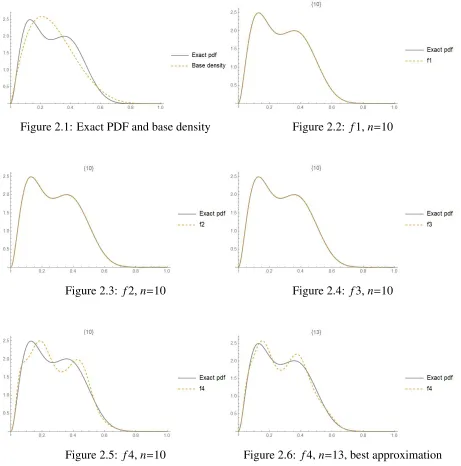
Figure 2.1: Exact PDF and base density Figure 2.2: f1,n=10
Figure 2.3: f2,n=10 Figure 2.4: f3,n=10
Figure 2.5: f4,n=10 Figure 2.6: f4,n=13, best approximation
It follows from the figures and Table 2.1 which includes the integrated squared differences
(ISD) between the exact and approximated pdf’s and the number of moments required to
ob-tain the approximate pdf’s, that types 1, 2 and 3 approximants can provide quite accurate
Figure 2.7: f5,ν=11,δ=0 Figure 2.8: f5,ν=17,δ=0, best approximation
Figure 2.9: f6,ν=9 Figure 2.10: f6, ν=12, δ=0, best approxima-tion
Table 2.1: Comparison of the ISD’s for different types and degrees
Type Degree # of moments ISD Degree # of moments ISD
1 10 10 0.00000231
2 10 10 0.0000281
3 10 10 0.0000336
4 10 10 0.0295788 13 13 0.0081179
5 11, 0 22 0.0008106 17, 0 34 0.0001887
6 9, 0 18 0.0215733 12, 0 24 0.0011875
7 5, 0 10 0.0133151 15, 0 30 0.0048238
approximations but require more moments than types 1,2 and 3. As for types 4, 6 and 7, the
resulting approximations are not as accurate.
2.4.2
Mixture of gamma pdf’s
Consider an equally weighted mixture of two gamma density functions with parameters (2,
2) and (9, 1) whose support is the positive half-line. We rescale the distribution using the
transformation
Y = X
σ,
whereσis the standard deviation of the mixture. On applying the transformation
Z= Y Y+1,
we obtain a random variable whose support is (0,1). We then apply the proposed methodologies
and compare the accuracy of the approximants.
It follows from the figures and Table 2.2 which includes the integrated squared differences
between the exact and approximated pdf’s, that in this case, the type 5 approximants provide
the most accurate approximations. Types 1, 2, 3 and 7 can also yield reasonably close
approx-imations. However, type 7 approximants require more moments than types 2 and 3 and the
resulting approximations are not as accurate.
1The bold-face numbers appearing in the tables correspond to the smallest integrated squared difference and
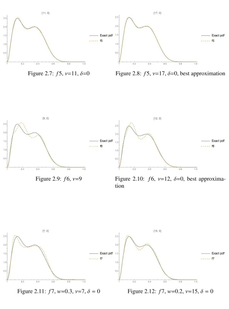
Figure 2.13: Exact density Figure 2.14: Transformed PDF’s
Figure 2.15: f1,n=10 Figure 2.16: f1,n=25, best approximation
Figure 2.17: f2,n=10 Figure 2.18: f2,n=12, best approximation
Figure 2.21: f5,ν=10,δ =0 Figure 2.22: f5, ν=11, δ = 0, best approxima-tion
Figure 2.23: f7,w= 0.1,ν=13,δ= 0 Figure 2.24: f7,w= 0.2,ν=11,δ=0
Table 2.2: Comparison of the ISD’s for different types and degrees
Type Degree # of moments ISD Degree # of moments ISD
1 10 10 0.0093 25 25 0.0011
2 10 10 0.0286 12 12 0.0047
3 10 10 0.0223 12 12 0.0036
5 10, 0 20 0.0004 11, 0 22 0.0002
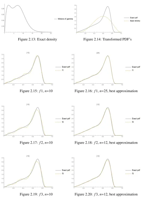
We can also obtain density approximants by truncating the distribution. Since FX(25) =
0.999937, which is nearly equal to one, we may focus on the interval (0,25). On applying
a linear transformation that maps the random variable X from (0,25) to (0,1) as well as the
proposed methodologies, we obtained the results that follow.
Figure 2.25: Truncated distribution Figure 2.26: Exact PDF and base density
Figure 2.27: f1,n=7 Figure 2.28: f2,n=11
Figure 2.29: f3,n=12 Figure 2.30: f4,n=11
It follows from the figures and Table 2.3 which includes the integrated squared differences
between the exact and approximated pdf’s, that the type 3 density approximant provides the
most accurate approximation. Types 1, 2 can also yield reasonably close approximations. As
Figure 2.31: f5,ν=17,δ =0 Figure 2.32: f7,ν=21,δ =0
Table 2.3: Comparison of the ISD’s for different types and degrees
Type Degree # of moments ISD
1 7 7 0.0002147
2 11 11 0.0000513
3 12 12 0.0000086
4 11 11 0.0105211
5 17, 0 34 0.0138683
7 21, 0 42 0.0093896
2.4.3
Mixture of normal pdf’s
Consider an equally weighted mixture of two normal distribution density functions with
pa-rameters (0, 1) and (5, 3). We rescale the mixture using the transformation
Y = X
σ,
whereσis its standard deviation. The support ofY is still (−∞,∞). On applying the
transfor-mation
Z = arctanY
π +
1 2,
we obtain a random variable whose support is (0, 1). We then implement the methodologies
and compare the results.
It follows from the figures and Table 2.4 that type 5 density approximants provide the most
accurate approximations. Types 1 and 2 can also yield reasonably close approximation. As for
Figure 2.33: Transformed PDF’s
Figure 2.34: f1,n=10 Figure 2.35: f1,n=23, best approximation
Figure 2.36: f2,n=10 Figure 2.37: f2,n=21, best approximation
Figure 2.40: f5,ν=9,δ= 0 Figure 2.41: f5,n=16,δ = 0, best approxima-tion
Figure 2.42: f7,w= 0.1,ν=11,δ= 0
Table 2.4: Comparison of the ISD’s for different types and degrees
Type Degree # of moments ISD Degree # of moments ISD
1 10 10 0.0113249 23 23 0.0023321
2 10 10 0.0302238 21 21 0.0014080
3 10 10 0.0304753 12 12 0.0195965
5 9, 0 18 0.0020256 16, 0 32 0.0000073
Alternatively, we can determine the approximants without standardizing the distribution,
select a normal density as base density and apply a type 1 approximation.
Figure 2.43: Mixture distribution PDF and base PDF
Figure 2.44: f1,n=40
Figure 2.45: f1,n=60 Figure 2.46: f1,n=90
Table 2.5: Comparison of the ISD’s for different degrees (Type 1 approximant)
Degree ISD
40 0.000302 60 0.000034 90 0.000002
It follows from the figures and Table 2.5 that in this case very accurate type 1
approxima-tions can be obtained using a large number of moments.
In conclusion, depending of the type of distributions being approximated, types 1, 2, 3 or 5
[1] Gajek, L. (1986). On improving density estimators which are not bona fide functions.
Annals of Statistics14(4), 1612–1618.
[2] Glad, I. K., Hjort, N. L., and Ushakov, N. G. (2003). Correction of density estimators that
are not densities.Scandinavian Journal of Statistics30(2), 415–427.
[3] Lindsay, B. G., Pilla, R. S. and Basak, P. (2000). Moment–based approximations of
distri-bution using mixtures: theory and applications.Annals of the Institute of Statistical
Mathe-matics52(2), 215–230.
[4] Provost, S. B. (2005). Moment–based density approximants.The Mathematica Journal 9,
727–756.
On Comparing Various Types of
Moment-Based Density Estimates
3.1
Introduction
Density approximants are obtained by making use of the exact moments of the target
distribu-tion. When it comes to estimating a density function on the basis of a sample of observations,
some of the previously introduced approaches can still be implemented by replacing the
pop-ulation moments by sample moments. The type 4 and type 6 approximants are not applicable
in this case since the moments µ4 andµ6 cannot be evaluated unless the exact distribution is
known.
These methodologies were applied to distributions whose support is the interval (0,1),
which, in some cases, required a transformation of variable. This chapter pertains to the
esti-mation of a density function from the sample moments associated with a set of observations.
In the case of samples, one can assign endpointsa andb to the underlying distribution ofY,
which can then be regarded as having a bounded support.
For example, we can let a equals to the minimum of the samples minus a constant times
the sample standard deviation and set the right endpointbsimilarly by adding a multiple of the
standard deviation to the maximum of the sample. Then, we let X = (Y −a)/(b−a), which
mapsY ∈(a,b) ontoX ∈ (0,1). After obtaining an estimate of the density function of the X,
we apply the inverse transformationY =(b−a)X+ato obtain a density estimate forY. Since
this is a linear transformation, the density estimates obtained before and after carrying out the
transformation have the same shape.
3.2
Simulated data
Before applying the methodologies to actual observations, we can assess their viability by
generating data sets from known distributions.
First, we select a certain mixture of density functions as our underlying distribution. Then
we fix a sample size and generate sample points from this distribution by making use of the
Monte-Carlo simulation technique. We then apply several of the methodologies introduced
in Chapter 2 by replacing the exact moments of the distribution with the sample moments
determined from the generated data. Our aim in this subsection is to verify the applicability of
the methodologies and determine their accuracy.
In this case, the sum of the squared differences (SSD’s) between the empirical cdf and the
estimated cdf is used as criterion to assess the accuracy of an estimate at the simulated points.
3.2.1
A mixture of beta pdf’s
Consider an equally weighted mixture of two beta density function with parameters (6,2) and
(3,9). We generated 500 sample points from this mixture. The base density is taken to be a
beta distribution that has the same first two moments as the sample moments. For comparison
purposes, plots of the kernel pdf and cdf estimates are included in certain graphs. The kernel
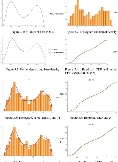
Figure 3.1: Mixture of beta PDF’s Figure 3.2: Histogram and kernel density
Figure 3.3: Kernel density and base density Figure 3.4: Empirical CDF and kernel CDF, (SSD=0.0832852)
Figure 3.5: Histogram, kernel density and f1 Figure 3.6: Empirical CDF andF1
Figure 3.9: Histogram, kernel density and f3 Figure 3.10: Empirical CDF andF3
Figure 3.11: Histogram, kernel density and f5 Figure 3.12: Empirical CDF andF5
Figure 3.13: Histogram, kernel density and f7, w=0.1
Table 3.1: Optimal density estimates of various types and SSD’s
Type Degree Number of moments SSD
1 10 10 0.0151
2 11 11 0.0138
3 11 11 0.0139
5 (8,0) 16 0.0545
7 (6,0) 12 0.0405
The degree(s) associated with the adjustments which are specified in Table 3.1, are the
minimizers of the sum of squared differences between the associated cdf estimates and the
empirical cdf (ECDF). The bold-face number corresponds to the smallest SSD and thus the
best density estimate. It is seen that in this case, a type 2 estimate (single polynomial) is the
most accurate. Types 1 and 3 can also provide excellent estimates. As for types 5 and 7, the
resulting density estimates are not quite as accurate; moreover, they require more moments.
3.2.2
A mixture of gamma pdf’s
Consider an equally weighted mixture of two beta density function with parameters (2, 2) and
(15, 1). We generated 500 sample points from this mixture. For this sample, min=0166412,
max=27.1662 and sd=6.53497.
After generating the sample points, we can obtain a density estimate for a distribution
whose support is for instance (0, max+sd). We then map the distribution onto the interval (0,
1) and take as a base density a beta distribution whose first two moments coincide with those
of the sample.
Figure 3.17: Kernel density and base density Figure 3.18: Empirical CDF and kernel CDF, (SSD=0.0944037)
Figure 3.19: Histogram, kernel density and f1 Figure 3.20: Empirical CDF andF1
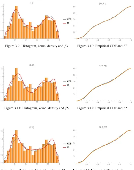
Figure 3.23: Histogram, kernel density and f3 Figure 3.24: Empirical CDF andF3
Figure 3.25: Histogram, kernel density and f5 Figure 3.26: Empirical CDF andF5
Figure 3.27: Histogram, kernel density and f7, w=0.1
Table 3.2: Optimal density estimates of various types and SSD’s
Type Degree # of moments SSD
1 12 12 0.0136
2 11 11 0.0144
3 11 11 0.0142
5 5, 0 10 0.1164
7 9, 0 18 0.0440
It is seen from Table 3.2 that in this case, types 1, 2 and 3 density estimates perform fairly
similarly in terms of accuracy, with type 5 being the least accurate. The type 1 estimate
advo-cated in Provost (2005) appears to be the most accurate.
3.3
Examples
We now model actual data sets whose underlying distribution is unknown.
3.3.1
The Bu
ff
alo snowfall data
This data set, which is available from the R library, contains 63 data points corresponding to
annual snowfall accumulation in inches as observed in Buffalo from 1910 to 1972; (min=25.0,
max=126.4, sd=23.7). Leta=min−sd= 1.03 andb=max+sd= 150.12.
If the density estimates are negative on certain subranges of the support, the algorithms
proposed by Gajek (1982) or Glad et al. (2003) can be applied. Alternatively, the negative
Figure 3.29: Histogram of the Buffalo snowfall data
Figure 3.30: kde (grey line) and base density Figure 3.31: Empirical CDF and kernel CDF, (SSD=0.0286895)
Figure 3.34: kde (grey line) and f2,n=11 Figure 3.35: ECDF and F2,n=11
Figure 3.36: kde (grey line) and f3,n=11 Figure 3.37: ECDF and F3,n=11
Figure 3.40: kde (grey line) and f7,ν=6,δ= 0 Figure 3.41: ECDF and F7,ν=6,δ= 0
Table 3.3: Optimal density estimates of various types and SSD’s
Type Degree # of moments SSD
1 10 10 0.0150
2 11 11 0.0260
3 11 11 0.0262
5 6, 0 12 0.0310
7 6, 0 12 0.0451
According to Table 3.3, the most accurate density estimate is of type 1 in this case.
More-over, this estimate requires fewer moments than the other ones.
3.3.2
The Old Faithful geyser data
This data set, which is available from the R library, contains 272 observations consisting of
durations between consecutive eruptions in minutes; (min=1.60, max=5.10, sd=1.14). Let
Figure 3.42: Histogram of the Old Faithful data
Figure 3.43: kde (grey line) and base density Figure 3.44: Empirical CDF and kernel CDF, (SSD=0.257145)
Figure 3.47: kde (grey line) and f2,n=9 Figure 3.48: ECDF andF2,n=9
Figure 3.49: kde (grey line) and f3,n=10 Figure 3.50: ECDF and F3,n=10
Table 3.4: Optimal density estimates of various types and SSD’s
Type Degree # of moments SSD
1 12 12 0.0732
2 9 9 0.1614
3 19 19 0.0276
5 (7,0) 14 0.0230
Table 3.4 indicates that the type 3 and 5 density estimates which require more moments
than the other types are the most accurate for this bimodal data set.
3.3.3
A large data set: US household income in 2016
This data set, which represents the mean US household income per city/village (excluding
zero values) is available from the website www.kaggle.com/datasets. It contains 32211
observations (min=5000, max=242857, sd=29873.1) that based on the US household incomes
in year 2016. Leta=0 andb= max+sd= 272730.1. As previously explained, this data was
mapped onto the interval (0, 1) before applying the various density estimation methodologies.
Figure 3.53: Histogram of the US household income data
It is seen graphically that in this case, the type 2 estimate provides the closest fit to the
empirical cumulative distribution of the data.
We conclude from this initial study that types 1, 2, 3 and 5 density estimates can, in most
of instances, model the data more accurately than kernel density estimates. However, more
Figure 3.54: kde (grey line) and base density Figure 3.55: Empirical CDF and kernel CDF, (SSD=0.0923982)
Figure 3.56: kde (grey line) and f1,n=19 Figure 3.57: ECDF and F1,n=19
Figure 3.60: kde (grey line) and f3,n=12 Figure 3.61: ECDF and F3,n=12
Figure 3.62: kde (grey line) and f5,ν=5,δ= 0 Figure 3.63: ECDF and F5,ν=5,δ= 0
Figure 3.64: kde (grey line) and f7,w=0.1,
ν=5,δ=0
Figure 3.65: ECDF andF7,w=0.1,
[1] Gajek, L. (1986). On improving density estimators which are not bona fide functions.
Annals of Statistics14(4), 1612–1618.
[2] Glad, I. K., Hjort, N. L., and Ushakov, N. G. (2003). Correction of density estimators that
are not densities.Scandinavian Journal of Statistics30(2), 415–427.
[3] Provost, S. B.(2005). Moment–based density approximants. The Mathematica Journal 9,
727–756.
Certain Types of Samples and their
Distributional Representativeness
4.1
Introduction
This chapter compares the stochastic simulation of samples from a given distribution via the
Monte Carlo technique with four deterministic (quasi-Monte Carlo) approaches, which consist
of making use of the percentiles resulting from a mapping with uniformly distributed discrete
points or the percentiles obtained from the mean, mode and median of the order statistics
as-sociate with the target distribution. Those four alternative types of samples which require that
the exact distribution be known, exhibit a more even coverage of the distributions. Such data
generation techniques could find applications in finance, actuarial science, engineering and
bi-ology among other fields of scientific investigation. Some relevant references on Monte Carlo
and quasi-Monte Carlo methodologies include Hammersley and Handscomb (1975),
Niederre-iter (1992), Caflish (1998), Robert and Casella (2004), Kalos and Whitlock (2008) and Metodi
et al.(2018).
4.2
Types of samples and criteria for determining their
dis-tributional representativeness
Our objective is to determine a distribution’s most representative sample of sizen. A group of
nrepresentative sample points should be such that their sample moments are similar to those
of the exact distribution up to a given order. Moreover, the empirical cumulative distribution
function based on thensample points should be relatively close to the exact cumulative density
function.
Suppose X that follows a given distribution with probability density function fX(x) and
cumulative distribution function FX(x), and let X1,X2, . . . ,Xn be a random sample from this
distribution. Let the order statistics be denoted as X(1),X(2), . . . ,X(n), the probability density
function ofX(k)being
fX(k)(x)=
n!
(k−1)!(n−k)!FX(x)
k−1(1−
F[x])n−kf(x) (4.2.1)
on the support of the distribution.
Lety1(k) be the expected value ofX(k), i.e.,
y1(k)= E[X(k)];
y2(k) be the mode ofX(k), i.e.,
y2(k)= argmax[fX(k)(x)];
y3(k) be the median of X(k), i.e., the 50th percentile of the distribution ofX(k); and
y4(k) be the (2k−1)/(2n)×100th quantile of fX(x).
Then, let
s2 =(y2(1),y2(2), . . . ,y2(n));
s3 =(y3(1),y3(2), . . . ,y3(n));
s4 =(y4(1),y4(2), . . . ,y4(n));
and s5= (x1,x2, . . . ,xn) be a given simple random sample of sizen.
These samples will be respectively referred to as types 1, 2, 3, 4 and 5 samples.
In this preliminary investigation, we make use of two distributions to determine which one
of the five types of samples is the most representative.
Four criteria are considered to determine the most representative sample of sizengenerated
from a given distribution.
Criterion 1: The first n sample moments, which according to Result 3 as stated in the
Introduction contain all the information included in the sample, are compared to the first n
exact moments by evaluating the sum of squared differences.
Criterion 2: The integrated squared difference between the resulting kernel density estimate
and the exact density is evaluated.
Criterion 3: The integrated squared difference between the empirical CDF (ECDF) and the
exact CDF is evaluated.
Criterion 4: The sum of the squared differences between the empirical CDF values
cor-rected with the factor n/(n+1) and the exact CDF values at the sample points. (Such points
are for instance plotted in Figure 4.5)
4.3
Assessment of distributional representativeness
4.3.1
Sample generated from a beta(2,5) distribution
First, we consider a sample of size 5 from a beta(2,5) distribution.
It is seen from Table 4.1 and Table 4.2 that the type 1 and 4 samples present some
advan-tages when compared to the other types.
Figure 4.1: Beta(2,5) PDF Figure 4.2: Samples of 5 types
Figure 4.4: Exact and empirical CDF’s for the 5 types of samples
sample moment of the type 1 sample happens to be the same as the exact one. Criterion 4
yields the smallest of the SSD’s for this type of sample. Type 4 samples are generated using
percentiles corresponding to equidistant cdf values. According to criteria 1 and 3, the type 4
sample outperforms the other samples.
In Table 4.3, the entries of Table 4.2 are divided by average of the values obtained for the
4 deterministic samples for each criterion and the row averages are evaluated for each type of
samples. A bold-face number appearing in a table corresponds to the most representative type
of sample in a given column.
According to Table 4.3, types 1 and 3 samples produce more accurate density estimates
since the corresponding averages are smaller.
Table 4.1: Relative errors between sample and exact moments
Number of moments 1 2 3 4 5
Type 1 Sample 0% – 8.53% – 20.34% – 33.48% – 46.57% Type 2 Sample – 8.48% – 19.76% – 32.41% – 45.45% – 52.72% Type 3 Sample – 2.55% – 12.01% – 24.10% – 37.20% – 50.04% Type 4 Sample – 1.33% −6.32% −13.90% – 23.78% – 35.03% Type 5 Sample 18.06% 22.61% 18.39% 7.71% −7.12%
Table 4.2: Rankings of the criteria for determine the most representative samples
Criterion 1 2 3 4 Average rank
Type 1 Sample 0.00028 (2) 0.0311 (4) 0.0026 (3) 0.0033 (1) 2.50 Type 2 Sample 0.00145 (4) 0.0201 (1) 0.0029 (4) 0.0126 (4) 3.25 Type 3 Sample 0.00047 (3) 0.0219 (2) 0.0024 (2) 0.0035 (2) 2.25 Type 4 Sample 0.00016 (1) 0.0293 (3) 0.0021 (1) 0.0111 (3) 2.00
Type 5 Sample 0.00333 (5) 0.1968 (5) 0.0107 (5) 0.0706 (5) 5.00
Table 4.3: Average of the criteria values
Criterion 1 2 3 4 Average
Type 1 Sample 0.47 1.22 1.04 0.43 0.79 Type 2 Sample 2.46 0.78 1.15 1.65 1.51 Type 3 Sample 0.80 0.86 0.97 0.46 0.77
4.3.2
Samples generated from a mixture of beta pdf’s
We now consider a sample of size 5 from an equally weighted mixture of two beta distributions
with parameters (8, 12) and (3, 15). In order to determine the most representative sample of
the distribution, the same four criteria are considered.
Figure 4.6: PDF of the mixture Figure 4.7: Samples of 5 types
Figure 4.9: Exact and empirical CDF’s for the 5 types of samples