An LRS based information system design for traffic survey data

(1)

NCDOT

Traffic Survey Unit

An LRS Based Information System Design

for Traffic Survey Data

By

Kent Taylor Larry Wikoff William Rasdorf

(2)

OUTLINE

1.0

INTRODUCTION

1.1

Background

1.2

Context

1.3

Objectives

1.4

Scope

1.4.1 Collection Elements

1.4.2 Reporting Elements

1.5

Report Organization

2.0

NCDOT LRS DATABASE DESIGN

2.1

Network Model

2.1.1 Topology

2.1.2 Geometry

2.1.3 State Maintained System

2.2

Attributes

2.2.1 Point Attributes

2.2.2 Segment Attributes

2.3

Network Position Identification

2.3.1 Mile Post Referencing

2.3.2 Offset Referencing

2.3.3 LRS Referencing

2.3.4 Coordinate Referencing

2.4

Spatial Data Integration Options

3.0

TRAFFIC SURVEY UNIT DATA

3.1

Spatial Data

3.1.1 Point Data Locations

3.1.2 Segment Data Locations

3.2

Attribute Data

3.2.1 Traffic Volume (AADT)

3.2.2 Single Unit Truck Volume

3.2.3 Multi Unit Truck Volume

3.2.4 Volume Seasonality

3.2.5 Vehicle Class Seasonality

3.2.6 Truck Weight Seasonality

3.3

Customers

3.4

Historical Data

4.0

DATABASE TABLES

4.1

Collection Data

(3)

4.1.2 Portable Vehicle Classification Counts Station Location

4.1.3 Permanent Volume Counts Station Location

4.1.4 Permanent Vehicle Classification Counts Station Location

4.1.5 Permanent Vehicle Class and Truck Weight Station Location

4.1.6 Manual Vehicle Class Count Location

4.1.7 Turning Movement Count Location

4.2

Reporting Data

4.2.1 Total Volume

4.2.1.1 Location

4.2.1.2 Segments

4.2.1.3 Values

4.2.2 SU Truck Volume

4.2.2.1 Location

4.2.2.2 Segments

4.2.2.3 Values

4.2.3 MU Truck Volume

4.2.3.1 Location

4.2.3.2 Segments

4.2.3.3 Values

4.2.4 Volume Seasonal Group

4.2.4.1 Location

4.2.4.2 Segments

4.2.5 Class Seasonal Goup

4.2.5.1 Location

4.2.5.2 Segments

4.2.6 Weight Seasonal Group

4.2.6.1 Location

4.2.6.2 Segments

4.3

Other Tables

5.0

PROGRAMS

5.1

ADM and LARS

5.2

Migration

5.3

Location Determination and Specification

5.4

Data Manipulation

5.5

Major Operations

5.5.1 Station Location

5.5.2 Reporting Segment Definition

5.5.2.1 Volumes

5.5.2.2 Seasonality

5.5.4 Data Editing

5.5.5 Publishing

5.6

AADT

5.6.1 Ownership

(4)

5.6.3 Business Process Enhancement

5.6.4 How AADT is Assigned

5.7

Data Access by the General Public

6.0

DATABASE SERVER ORGANIZATION

7.0

IMPLEMENTATION

8.0

ROLES AND RESPONSIBILITIES

8.1

LRS

8.2

GIS

8.3

World Wide Web

9.0

CONCLUSIONS

(5)

List of Tables

Table 3.1: Multi Segment Attribute Illustration for AADT Data Table 3.2: Traffic Volume Tables

Table 4.1: Database Table Format

(6)

List of Figures

Figure 1.1: LRS Data Storage and Delivery Figure 2.1: Graphical Highway Network Model Figure 2.2: Geometry of the Network Model Figure 2.3: Points on the Network Model Figure 2.4: Segments on the Network Model

Figure 2.5: Specifying a Point Location Using Mile Post Referencing Figure 2.6: Specifying a Point Location Using Offset Distance

Figure 2.7: Specifying a Point Location Using LRS Offset Figure 2.8: Specifying a Point Location Using Coordinates Figure 2.9: Snapping Coordinates to the Roadway Network Figure 5.1: Data Collection and Reporting

Figure 5.2: Station Location Matching Illustration Figure 5.3: Close Matching of Two Counts

(7)

1.0

INTRODUCTION

The primary function of the Traffic Survey Unit (TSU) is to collect transportation data and to format it in a meaningful manner. The unit may be viewed as a traffic data warehouse. This data can then be published so that it may be used by other NCDOT units and by outside agencies and interested parties. Approximately 90 percent of the data is specific to traffic volumes, vehicle types, and vehicle weights.

In addition to storing data, the TSU analyzes data to derive traffic and travel statistics that are of use to others. In the future, TSU would like to provide on-line access to as much of its data as possible for all those who might be interested in traffic information. Although the unit undertakes many activities, the one of interest in this report is to define the information system design for a key subset of traffic survey data.

1.1

Background

Handling data is a difficult task as evidenced by the emergence of an entirely new discipline called information technology which was created to formalize this task. Of particular importance in data handling are:

• data collection

• data storage

• data quality maintenance and enhancement

• data delivery

This report focuses on data storage and delivery.

The TSU warehouses a variety of data in multiple formats. These can be simplified into two main categories:

• paper

• electronic

The electronic data encompasses files, disks, tapes, CDs, etc. The paper data includes completed data collection forms, paper printouts, and annotated maps. The future goal of the TSU is to move increasingly toward electronic formats. In particular the Unit seeks to:

• develop a comprehensive database (and to ultimately make its data available via the world wide web). [data storage]

• allow presentation of data using a GIS display. [data delivery]

• allow presentation of data using the world wide web. [data delivery] These three goals focus on the data storage and data delivery tasks of the Unit.

(8)

Presently, many NCDOT Units have their own location referencing method and most differ to some extent. As a result, department wide data sharing and exchange are significantly inhibited because of the need to write location referencing translation programs. Additionally, data analysis using diverse data sets is inhibited. Thus, multi-disciplinary queries such as “find all accidents where the pavement condition rating is low and the AADT is high (insert some appropriate values here)” are not presently easy to resolve. Such a query would require data from PMU, TSU, and TE. The data sets of these units and branches are not currently well linked. The purpose of the LRS is to make this less difficult.

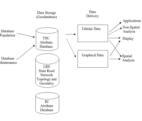
The new LRS will provide a common, standardized highway network on which any NCDOT Unit may overlay its data. The GIS Unit will maintain the network topology and geometry and each unit will maintain their own attribute data as shown in Figure 1.1. The LRS is the network and TSU data is event data associated with the LRS.

Figure 1.1: LRS Data Storage and Delivery

Applications

Display

Spatial Analysis Graphical Data

Tabular Data

LRS State Road

Network Topology and

Geometry TSU Attribute Database

Database Maintenance

Database Population

Data Storage (Geodatabase)

Data Delivery

Non Spatial Analysis

(9)

In Figure 1.1 the GIS Unit maintains the LRS State Road Network Topology and Geometry which constitutes the Geodatabase. The GIS Unit is responsible for the network while others are responsible for their data. This is the preferred approach as no one is as capable of taking care of the data as the Unit from which it originated.

1.2

Context

The LRS itself is now under development and is an ongoing and evolving project. Such development may, over time, cause some of the content of this document to change as the LRS evolves.

This document relates to the 1.X data model and series of releases for the LRS. It is a study intended to show how to integrate TSU with the new LRS. This document represents a recommended design that is to be used as a basis for an implementation. It is not yet a specific project proposal to develop a product. Thus, it serves as an advising resource and best practice document but does not serve as a project charter of the GIS Unit.

The normal business process for the GIS Unit would encompass the development of numerous documents including a Project Request Document, a Project Charter, and a Project Formal Agreement. This report lays the foundation for a Project Request Document which would enable the GIS Unit to assess the needs of TSU and respond with what could be done and how. Thus, this report helps to define the overall vision and goal of TSU.

1.3

Objectives

One objective of this report is to present the general database design for Traffic Survey Unit data (TSU Attribute Database as shown in Figure 1.1) that will be made available via the NCDOT LRS. This document will support the future integration of the TSU database schema into the LRS database. In addition, this report describes the processes (additional programs and programming) needed to implement the database population and maintenance activities.

This report defines what we refer to as the core data items to be initially implemented. The ultimate LRS database is in no way limited to these data items and, in fact, is expected to expand and evolve over time. However, at present, this report describes material that is broad enough in scope to provide useful and meaningful data, yet it is not as broad as to limit implementation or to require excessive resources. It is a target that can be successfully met in a reasonable time frame with low risk and high payoff.

1.4

Scope

Linear referencing of traffic data will be divided into two categories:

• Collection Elements

• Reporting Elements

Collection refers to the acquisition of data. Reporting refers to the dissemination of data.

(10)

Reporting elements are a representation of the results of one or more analyses from a collection element translated to a segment on the linear highway system. Where collection elements are primarily point references, reporting elements are primarily segment references. Reporting elements are the initial TSU data items to be made available to the public through the LRS.

1.4.1 Collection Elements

Point elements to support data collection activities are as follows:

• PTC (Portable Volume Counts) - Station Identifier.

• PVC (Portable Vehicle Classification Counts) - Station Identifier.

• ATR (Permanent Volume Counts) - Station Identifier.

• AVC (Permanent Vehicle Classification Counts) - Station Identifier.

• WIM (Permanent Vehicle Class and Truck Weight) - Station Identifier.

• MC (Manual Classification - Manual Vehicle Class) - Station/Event Identifier.

• TM (Turning Movement - Intersection movement counts and count data on approaches to the intersection) - Station/Event Identifier.

The first 6 types of counts shown above are collected at points located between intersections. The turning movement count, on the other hand, is always located directly at an intersection. However, some of these intersections are not on the State highway system. This presents a problem in that the LRS presently handles only the state highway network. This problem needs to be addressed in the final design. It does not initially need to be addressed because the evolution of the LRS may be such that the problem is resolved before it becomes a significant problem. For the present this is handled simply by storing the data using the turning pavement count identifier and leaving the intersection identifier blank.

1.4.2 Reporting Elements

Segment elements to support data reporting activities are as follows:

• Volume (AADT) - Total Volume (in vehicles per day) - Source Data Identifier.

• Single Unit (AADVT_SU) Trucks - SU Truck Volume (in vehicles per day) - Source Data Identifier.

• Multi Unit (AADVT_MU) Trucks - MU Truck Volume (in vehicles per day) - Source Data Identifier.

• Volume Seasonality - VOLUME Group or Station Identifier.

• Vehicle Class Seasonality - VC Group or Station Identifier.

• Truck Weight Seasonality - TWR Group or Station Identifier.

(11)

1.5

Report Organization

This report contains the following major sections:

• NCDOT LRS Database Design

• TSU Data

• Database Tables

• Programs

• Database Server Organization

• Implementation

• Roles and Responsibilities

This report first addresses and explains the NCDOT LRS database design. It then describes the data that the Traffic Survey Unit handles, collects, stores, and processes. Two issues are addressed in particular: spatial location and attribute values. Traffic Survey data items are then described in detail in the Traffic Survey Database Tables Section. The design of the database tables is also presented.

The next portion of the report addresses various business processes that use the data in the Programs Section. The major programs that need to be written to achieve the database design (previously described) are discussed. The report then focuses on the data that is to be stored using Oracle, including which data is public vs. private, and how that data is organized on the server. Trade-offs between a database (tabular) and a GIS (graphical) approach are discussed.

(12)

2.0

NCDOT LRS DATABASE DESIGN

The purpose of the LRS is to robustly and accurately model the state’s highway network.

2.1

Network Model

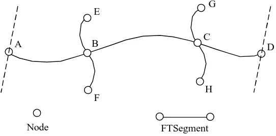
Figure 2.1 presents a graphical model of a highway network using the graphical elements of lines and circles. We refer to the circles as nodes and the linear elements between them as FTSegments. The linear elements are not straight but may be of any shape. Thus, in Figure 2.1 AB, BC, CD, EB, BF, GC, and CH are FTSegments and A, B, C, D, E, F, G, and H are nodes. These are the components of the LRS network model.

The components of the LRS model are entirely different from the graphical display elements shown in Figure 2.1. A, B, C, D, E, F, G, and H are circles and AD, EF, and GH are lines. These are graphical display elements whether they be in black and white or in color. The graphical display corresponds to the underlying LRS database model.

In this report we are concerned with the highway network model. Graphical display is of secondary interest. Thus, our focus is on the database and the network model it uses to achieve the spatial representation of the linear data associated with the highway network. Topology and geometry are two essential components of the network model.

Figure 2.1: Graphical Highway Network Model

2.1.1 Topology

Topology embodies the connectivity of the network. The Topology of the state road network is captured in the LRS through the use of nodes and FTSegments. A node occurs where two lines intersect (B, C), at a dead end of a line (E, F, G, H), or at a state or county boundary (A, D). An FTSegment is the segment between two nodes (AB, BC, CD, BE, BF, CG, CH). We “connect” nodes and FTSegments through references to each other using an identifier. We can then answer queries related to the connectivity of the network.

2.1.2 Geometry

The geometry of the state road network is captured in the LRS by storing the length of the FTSegments. In a linear system position in space is determined by length, or position along a portion of the network, rather than by absolute position on the earth. Thus, GPS coordinates are

A

FTSegment Node

F B

H C

D G

(13)

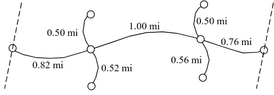
length measurements of the network elements are stored and distances can be determined using these. The length of the FESegments in Figure 2.1 are shown in Figure 2.2.

Figure 2.2 Geometry of the Network Model

It should be noted that here we are discussing the modeling of geometry in a relational database rather than in a GIS. While length is the item stored in the relational database to specify geometry, shape is what is stored in a graphical model of geometry in a GIS.

2.1.3 State Maintained System

The purpose of the network model is to create an accurate representation of the physical roadway system. In particular, the focus of the LRS is on modeling the State Maintained Roadway System. As a result, only state maintained roads are initially planned to be incorporated in the database. Thus, FTSegments represent segments on the State Road System and FTRPs represent intersections of roads on the System.

This presents what appears to be a problem for TSU. Often, Turning Movement counts occur at the intersection of a state road with a non-state road or at the intersection of two non-state maintained roads. If such roads are not represented in the system then it is not the case that TM counts are taken at an FTRP. However, it is expected that the LRS will evolve so that FTRPs can be inserted at these pointes because it is a future desire to have non-state maintained roads added to the system.

At the present time this problem can be handled in the database simply by providing a turning movement count identifier and not specifying an FTRP. This results in an incomplete record but it still enables the system to record all the data.

2.2

Attributes

The items placed onto the network are referred to as attributes. Attributes are characteristic of an object that describe it. Attributes of different components of the highway network include speed limit, traffic volume, number of lanes, etc.

2.2.1 Point Attributes

One attribute type is a point attribute. A point may represent a physical entity such as a count station, a sign, a culvert, a railroad crossing, etc. A point attribute may also represent a conceptual entity such as a county boundary or other political entity. Both physical and conceptual entities retain a position on the network. Figure 2.3 illustrates points A and D as

0.82 mi _{0.52 mi} 0.50 mi

0.56 mi

(14)

representing county boundaries, point 1 as representing a rail road crossing, and point 2 as representing a culvert, for example.

Figure 2.3 Points on the Network Model

Point attribute position in the LRS is determined relative to FTSegments. To identify a position requires the specification of an FTSegment identifier, an end node (of the FTSegment) identifier, and an offset distance from the specified end node to the point attribute under consideration. That location may in fact be directly on the reference point itself and this is indicated by having an offset distance of zero. Offset referencing is further discussed in Section 2.7 below. The collection points of the TSU data set are point attributes.

2.2.2 Segment Attributes

A second attribute type of interest in a transportation network is a segment attribute. A segment attribute may represent a physical entity such as pavement, a guard rail, a shoulder, a median, etc. A segment attribute may also represent a non physical item such as speed limit, AADT, name, etc. Each of these extends along a length of the network at some linear location. Thus, like point attributes, a segment attribute also retains a position on the network, although it is a linear position rather than a point position.

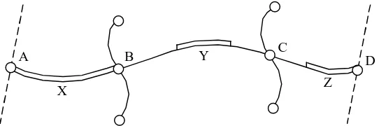
Figure 2.4 illustrates the concept of segment attributes. The segment identified as X extends from node A to node B and encompases the entire FTSegment AB. The segment identified as Y extends from some point on FTSegment BC to some other point on FTSegment BC, neither of which lies at either end of the segment. Finally, the segment identified as Z has one end that corresponds to node D, but its other end lies at some point along FTSegment CD.

Figure 2.4: Segments on the Network Model

Linear position is also determined relative to FTSegments. In fact, it is determined in exactly the same way as for point attributes because the boundary of each segment consists simply of two points delineating each of its ends.

X A

X X

2

X D

X 1

A

X

B

Z C

(15)

The reporting elements of the TSU data set are segment attributes.

2.3

Network Position Identification

Network position identification means to identify where on the network an attribute is positioned. This report describes four ways that is commonly done. These are:

• Mile Post Referencing

• Offset Referencing

• LRS Referencing

• Coordinate Referencing

2.3.1 Mile Post Referencing

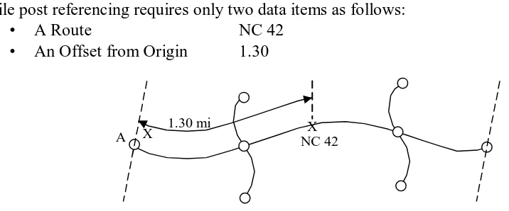
Mile post referencing is a common method of specifying and identifying locations within and among DOTs. Figure 2.5 illustrates the use of mile post referencing to refer to a point X on the example network of Figure 2.1.

Mile posting is a conceptual measurement system where distance is measured from the start of a road within a county. For interstate roads, however, mile posting is measured from the start of a road within the entire state. If a road does not cross a state or county boundary, mile posting begins at the point at which the road starts. Increasing mileage generally occurs in easterly and northerly directions. In Figure 2.5 the milepost of point X is 1.30 miles on NC 42. In this case, the mile posting begins at point A which is a county boundary.

Mile post referencing requires only two data items as follows:

• A Route NC 42

• An Offset from Origin 1.30

Figure 2.5: Specifying a Point Location Using Mile Post Referencing

Mile post referencing presents severe challenges for location referencing. In actuality it is a form of referencing that is not intuitive and is not referenced to anything predictable or expected. Furthermore, when a section of a road is relocated, the mileposts of all of the features north and east of it will change. It is difficult to develop database systems when the locations of attributes appear to change. Thus, this form of referencing has significant shortcomings.

2.3.2 Offset Referencing

Offset referencing is the primary method of specifying and identifying location in the field. It is also an effective way to specify location in a database and is well suited to the LRS. That is, it

X

NC 42

1.30 mi _X

(16)

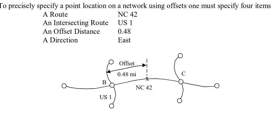
can easily be implemented in the LRS. Offset referencing ties the location of a point to the location of some other known point. Refer to Figure 2.6 for an example.

To precisely specify a point location on a network using offsets one must specify four items:

A Route NC 42

An Intersecting Route US 1 An Offset Distance 0.48

A Direction East

Figure 2.6: Specifying a Point Location Using Offset Distance

The route number is the identifier of the route on which the point lies. The intersecting route is a route that crosses the route on which the data point lies. This crossing defines the intersection that is used as the reference point for the measurement. The offset then is the mileage distance from the identified intersection to the location in question (along the route), given to hundredths of a mile, in the specified direction.

Note that the example shown in Figure 2.6 is that of locating a point. A segment would be identified similarly using two end points. The segment end points may be measured from the same end intersection or they may be measured from a different intersection.

2.3.3 LRS Referencing

LRS referencing is a specialized form of offset referencing. It is the method used in the new NCDOT LRS database. The reader is referred to Figure 2.7 for an example.

Figure 2.7: Specifying a Point Location Using LRS Offset

B

C

FTSeg 403621 Offset

0.48 mi x B

C

NC 42 Offset 0.48 mi

x

(17)

To precisely specify a point location on a network using LRS referencing one must specify three items:

An FTSegment Identifier 403621 (between nodes B and C) An FTRP Identifier B

An Offset Distance 0.48

The FTSegment identifier represents the FTSegment on which the point lies. The FTRP identifier represents the end node from which the offset is measured. The offset then is the mileage distance from the identified node to the point location of interest along the FTSegment, given to hundredths of a mile.

Note that the example shown in Figure 2.7 locates a single point. A segment would be represented similarly using two end points. The segment end points may be measured from the same end node or they may be measured from different end nodes.

2.3.4 Coordinate Referencing

Numerous NCDOT Units have access to and use GPS units. The TSU is one that expects to make significant use of GPS units in the future. These are devices that identify the geodetic (latitude, longitude, elevation) or geographic (N, E, Z) coordinates of a point on the surface of the earth. To precisely specify the location of a point on the earth’s surface requires exactly these 3 coordinate values.

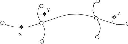
However, one difficulty with points is that they may not, when loaded into ArcGIS, appear directly on the lines that represent roads. Figure 2.8 illustrates this situation.

Figure 2.8: Specifying a Point Location Using Coordinates

Three example points are shown in Figure 2.8. Point X had coordinates that placed it directly on the roadway network. However, points Y and Z did not fall directly on the roadway network even though during measurement the field technician stood directly on the road to collect the coordinate data.

The reasons for the point and line not matching are numerous. The technology, accuracy, and precision of the instruments used to collect GPS data can vary widely. Thus, the GPS coordinates are not exact even though they may be reasonably accurate and precise. Second, the technology of placing a road in either CAD or GIS software is not completely accurate either. Thus, it is possible that the road, the coordinates, or both are inaccurately positioned. It is no wonder then that they might not match up visually. That is why we assume they do match if they

*

X

Y

(18)

are “close,” i.e., within a tolerance of each other. The process of determining that two points are close enough to each other to be the same point is referred to as “matching.”

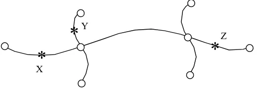
What has to happen when situations like Y and Z occur is that they must be “snapped” to the line work. That is, they must simply be “put” somewhere on the line. This process of moving them from off the line to on it is called snapping. Snapping algorithms usually are produced in GIS software and they usually move a point to the line along a path perpendicular to the road. That is, they move from where they are to the closest possible point on the line. Figure 2.9 shows the GPS locations of the points from Figure 2.8 after they have been snapped to the line work.

Figure 2.9: Snapping Coordinates to the Roadway Network

There are thus two key operations that are needed by the TSU. The first is snapping and the second is matching.

2.4

Spatial Data Integration Options

The LRS enables the NCDOT GIS Unit to maintain both the topology and the geometry of the State highway network. In this manner, one organizational Unit is responsible for the completeness and correctness of this network. But other Units may attach their data to the network and obtain the following benefits:

• They are not responsible for maintaining the network.

• They are responsible for maintaining only their data.

• Their data is combined with the data of everyone else using the LRS.

• Their data is available for multi attribute query and analysis via a GIS.

• Their data is readily available for use by customers and others.

• There is fast ad-hoc access to all data.

• There is access to versatile mapping resources.

There are two integration paths for external customers with respect to the LRS as follows:

• Convert their location referencing method and attribute database structure to that of the LRS.

• Maintain their current location referencing system and database structure and translate between systems when needed.

The advantages of conversion include all of those mentioned above plus the following:

• The connection to the LRS can be real-time.

• Tools for data maintenance can be made available and maintained by the GIS Unit.

*

X

Y

(19)

• All customers have a uniform set of tools for accessing all data.

• Direct access to a highly reliable and accurate highway network.

The disadvantages of conversion are as follows:

• Reliance on the GIS Unit for the highway network.

• Reliance on the GIS Unit for the tools to use the system.

• Transition of TSU customers to LRS to access data.

• For customers not using the LRS, conversion software will be required to access TSU data.

The advantages of translation are as follows:

• The customer's data remains detached and removed from other data and access by other users.

The disadvantages of translation are as follows:

• Determining who will write the conversion software.

• Time delay while translation software is designed, implemented, tested, and placed into production.

• The connection is not real time.

• The translation will inherently contain errors.

(20)

3.0

TRAFFIC SURVEY UNIT DATA

This data consists of spatial traffic survey data that is on the LRS. In fact, these tables show how it is placed on the LRS.

3.1

Spatial Data

It has been noted that point and segment data are the primary forms of data applied to the network. Point data occurs at a specified point. Multiple points may exist on a given FTSegment or on the Road Segments of which the FTSegment is comprised. Segment data, however, can occur over less than one, on one, or on multiple FTSegments. If it occurs over less than one FTSegment then its extent is specified on the underlying Road Segments.

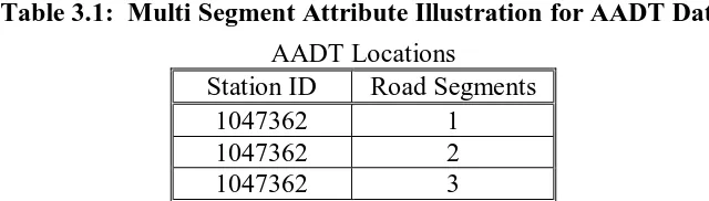
Table 3.1: Multi Segment Attribute Illustration for AADT Data

AADT Locations

Station ID Road Segments

1047362 1

1047362 2

1047362 3

Table 3.1 illustrates one set of road segments over which a particular station’s data might apply. In the example shown, the AADT data from station 1047362 applies to three Road Segments whose IDs are 1, 2, and 3. Thus, station data can span multiple Road Segments and could also span multiple FTSegments. It is also the case that AADT might exactly match the extent of a single FTSegment exactly. Additionally multiple AADTs might occur on different portions of the same FTSegment.

3.1.1 Point Data Locations

These data items represent the point locations at which counts are taken. These are referred to as collection elements. The following abbreviations and acronyms define TSU point data. These were previously described in Section 1.3.1.

• PTC

• PVC

• ATR

• AVC

• WIM

• MC

• TM

3.1.2 Segment Data Locations

(21)

• AADT

• AADVT_SU

• AADVT_MU

• Volume Seasonality

• Vehicle Class Seasonality

• Truck Weight Seasonality

3.2

Attribute Data

This data consists of the attribute values for the point and segment data locations previously defined. This is public data that is to be made available on the LRS. This is the data that the TSU seeks to make readily available to its customers.

3.2.1 Traffic Volume (AADT)

The AADT is the annual average daily traffic for all vehicles. This value is an estimate of the average of all typical days throughout the year. The AADT value is derived through a series of processes. These are further discussed in Section 5.6.

Units: Vehicles per day

Data Type: Integer

Typical Range of Values: 10 - 170,000

Table Name: AADT

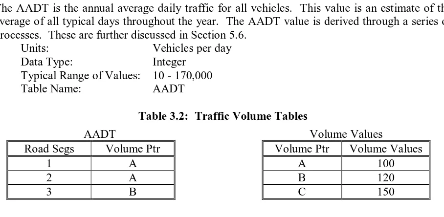
Table 3.2: Traffic Volume Tables

AADT

Road Segs Volume Ptr

1 A

2 A

3 B

Volume Values

Volume Ptr Volume Values

A 100

B 120

C 150

This data tells us the AADT volume attribute values at any segment location on the network. This is how reporting elements are implemented in the LRS. Each road segment possesses a volume pointer that indicates a volume value for that road segment. The extent over which that volume value applies is the number of contiguous road segments that possess that value pointer. Thus, in Table 3.2 the value of 100 vehicles per hour occurs on both road segments 1 and 2.

(22)

3.2.2 Single Unit Truck Volume

The AADVT_SU is the annual average daily vehicle traffic for single unit trucks. This value is an estimate of the average of all typical days throughout the year.

Units: Single unit trucks per day

Data Type: Integer

Table Name: SUTV

3.2.3 Multi Unit Truck Volume

The AADVT_MU is the annual average daily vehicle traffic for multi unit trucks. This value is an estimate of the average of all typical days throughout the year.

Units: Multi unit trucks per day

Data Type: Integer

Table Name: MUTV

3.2.4 Volume Seasonality

Volume seasonality provides a description of the pattern of travel on a facility throughout the year. It accounts for volume changes as seasons change and captures variations in seasonal travel.

Current

Units: Groups

Data Type: Integer

Typical Range of Values: 1 - 7 and 11 - 14

Table Name: AADT

Proposed

Units: Groups

Data Type: Enumerated

Typical Range of Values: 01-99

Table Name: VOLUMEGROUP

3.2.5 Vehicle Class Seasonality

The vehicle class seasonality accounts for differences in vehicles themselves on a highway. This represents a factor used to account for vehicle class.

Units: Groups

Data Type: Integer

Typical Range of Values: 01-99

Table Name: VCGROUP

3.2.6 Truck Weight Seasonality

Truck weight seasonality groups road segments by truck weight.

Units: Groups

Data Type: Integer

(23)

3.3

Customers

The TSU has a number of primary customers. The first is the GIS Unit of the NCDOT. In particular this is the Road Inventory Information System Section (RIIS). This section utilizes AADT data from TSU to support FHWA data reporting requirements. The second TSU customer is other NCDOT units. The third are the NCDOT division engineers. Finally another customer is the general public.

The TSU expects that some of their customers would readily make use of the TSU LRS data. Others would prefer access to data in more traditional formats. Initially it is expected that the RIIS would prefer the former but the general public might prefer the latter form of access. There would be a transition for other NCDOT units and for the division engineers.

3.4

Historical Data

It should be noted that data is time dependent. Historically this has been handled by having archivable hard copies of maps and archivable files of data periodically stored in cabinets or on CD’s. It is recommended that this practice be continued during the initial LRS startup. That is, it is recommended that periodic backups be made of the data.

(24)

4.0

DATABASE TABLES

This section defines the structure of the schema design for the TSU data. The schema design is in line with the structure of the database tables for RIIS. That is, the TSU design adopts the basic table format and schema design of the LRS as it has been defined and developed. Thus, TSU is converting its data to the LRS format. It is not maintaining a separate format that requires conversion programs.

This report includes a relational database schema. The schema is presented to the reader using two formats. In one format database tables are illustrated by identifying the table name along with its primary key(s) and attributes as follows.

TABLE NAME (Primary Key, Attribute 1, Attribute 2, Attribute 3, …, Attribute n)

When using this format a definition is provided for each attribute and a description is also provided for the overall content and meaning of the data contained in the table. The attributes are presented in bold face so that they can easily be identified.

In the second format, actual tables with representative data are presented. These tables are intended merely as a guide to enhance the illustration, where necessary, and the reader's understanding of the schema. They are provided in the following form. When using this format, each cell in each table contains data values.

Table 4.1: Database Table Format

TABLENAME

Primary key Attribute 1 … Attribute n

Both of the formats presented here complement and mirror each other. The second allows us to present example data that often further clarifies the reader's understanding of the schema design. This second format, however, will only be used when such clarification is absolutely necessary.

4.1

Collection Data

This report section presents the database tables that are necessary to store the TSU collection data. Each collection item that was previously discussed is presented.

4.1.1 Portable Volume Counts Station Location

This table identifies the physical location of a PTC count station which is referred to as a coverage volume identifier. A PTC count station is a point location on the highway network. The offset method is used for its specification.

FPL_PTC_REC (CVRG_VLM_ID, FTSegID, FTRPID, Offset Distance)

(25)

FTSegID – Statewide unique LRS segment identification number assigned to this network segment.

FTRP – The statewide unique LRS node identifier assigned to the network node from which the location of the CVRG_VLM_ID is measured.

Offset Distance – The distance between the location of the CVRG_VLM_ID being considered and an FTRP at one end of the given FTSegID.

4.1.2 Portable Vehicle Classification Counts Station Location

This table identifies the physical location of a PVC (Vehicle Classification) count station. A PVC count station is a point location on the highway network. The offset method is used for its specification.

FPL_PVC_REC (CVRG_CLS_ID, FTSegID, FTRPID, Offset Distance)

CVRG_CLS_ID – The station identifier; a numerical value that combines county and station ID number in one overall value; unique statewide. 01001221 is an identifier wherein 010 represents Bucombe County and 01221 represents the station sequence number, unique county wide.

FTRP – The statewide unique LRS node identifier assigned to the network node from which the location of the CVRG_CLS_ID is measured.

Offset Distance – The distance between the location of the CVRG_CLS_ID being considered and an FTRP at one end of the given FTSegID.

4.1.3 Permanent Volume Counts Station Location

This table identifies the physical location of an ATR (Automatic Traffic Recorder) station. An ATR count station is a point location on the highway network. The offset method is used for its specification.

FPL_ATR_REC (CNTNS_VLM_ID, FTSegID, FTRPID, Offset Distance)

CNTNS_VLM_ID – The station identifier; a character string value that combines county and station ID number in one overall value; unique statewide; and preceded by the letter A. A9101 is an identifier wherein the letter A indicates an ATR station, 91 represents Wake County, and 01 represents the station sequence number, unique county wide.

FTRP – The statewide unique LRS node identifier assigned to the network node from which the location of the CNTNS_VLM_ID is measured.

Offset Distance – The distance between the location of the CNTNS_VLM_ID being considered and an FTRP at one end of the given FTSegID.

4.1.4 Permanent Vehicle Classification Counts Station Location

This table identifies the physical location of an AVC (Permanent Vehicle Classification) station. An AVC count station is a point location on the highway network. The offset method is used for its specification.

FPL_AVC_REC (CNTNS_CLS_ID, FTSegID, FTRPID, Offset Distance)

(26)

FTRP – The statewide unique LRS node identifier assigned to the network node from which the location of the CNTNS_CLS_ID is measured.

Offset Distance – The distance between the location of the CNTNS_CLS_ID being considered and an FTRP at one end of the given FTSegID.

4.1.5 Permanent Vehicle Class and Truck Weight Station Location

This table identifies the physical location of WIM stations. A WIM count station is a point location on the highway network that is regularly monitored and has a station identifier. Because the location is permanent it is sufficient to have a station ID. The offset method is used for its specification.

FPL_WIM_REC (MNL_WIM_ID, FTSegID, FTRPID, Offset Distance)

MNL_WIM_ID – The station identifier; a character string value that combines county and station ID number in one overall value; unique statewide; and preceded by the letter W. W7413 is an identifier wherein the letter W indicates a WIM station, 74 represents Polk County, and 13 represents the station sequence number, unique county wide.

FTRP – The statewide unique LRS node identifier assigned to the network node from which the location of the MNL_WIM_ID is measured.

Offset Distance – The distance between the location of the MNL_WIM_ID being considered and an FTRP at one end of the given FTSegID.

4.1.6 Manual Vehicle Class Count Location

This table identifies the physical location where a manual vehicle class count is taken. An MC station is a point location where an individual performs a manual vehicle classification count on the highway network. Multiple counts may be taken at the same location but these would receive different identifiers. The offset method is used for its specification. It should be noted that StationID is not a sufficient identifier for this data item. Instead, each count must have a unique identifier because the counts may be taken in different locations.

FPL_MC_REC (MNL_CLS_ID, FTSegID, FTRPID, Offset Distance)

MNL_CLS_ID – The count identifier; a character string value that combines the year the count was taken, the initials MC, and a sequence number; unique statewide. 04MC0006 is an identifier that indicates a 2004 count identified as 0006.

FTRP – The statewide unique LRS node identifier assigned to the network node from which the location of the MNL_CLS_ID is measured.

Offset Distance – The distance between the location of the MNL_CLS_ID being considered and an FTRP at one end of the given FTSegID.

4.1.7 Turning Movement Count Location

(27)

directly on an FTRP (see discussion in Section 2.1.3 for further clarification of this point). No offset distance is required. It should be noted that StationID is not a sufficient identifier for this data item. Instead, each count must have a unique identifier because the counts may be taken in different locations.

Turning_REC (TM_ID, FTRP)

TM_ID – The count identifier; a character string value that combines the year the count was taken, a TM (turning movement) indicator, and a sequence number; unique statewide. 04TM0006 is an identifier that indicates a 2004 TM count number 0006.

FTRP – The statewide unique LRS node identifier assigned to the network node at which this count is being taken.

4.2

Reporting Data

This report section presents the database tables that are necessary to store the TSU reporting data. Each reporting item that was previously discussed is presented.

4.2.1 Total Volume

4.2.1.1 Location - This table stores the physical location of a segment of road for which an AADT quantity value has been specified. The table indicates where along the length of this particular FTSeg the value lies.

FPL_AADT_REC (AADT_ID, FTRPID, FTSegID, FRM_DSTNC_QTY, TO_DSTNC_QTY)

AADT_ID – The AADT volume identifier. This is an arbitrarily assigned numerical value for this AADT volume location.

FTRPID – The statewide unique LRS node identifier assigned to the network node from which the location of both the beginning and end of the AADT value is measured.

FRM_DSTNC_QTY – The distance from one end of the AADT value to the FTRPID reference point.

TO_DSTNC_QTY – The distance from the other end of the AADT value to the FTRPID reference point.

4.2.1.2 Segments - This table identifies the underlying set of road segments that comprise this AADT segment.

FPL_AADT_XREF (RDSeg_ID, AADT_ID)

RDSeg_ID - Statewide unique LRS segment identification number assigned to this road segment. Multiple road segments may constitute a single AADT segments.

(28)

4.2.1.3 Values - This table stores the AADT value that is assigned to a segment of road. This table contains the most recent published data. If data is not available in a given year the data from the previous year is used. Thus if a station was not counted in 2006, for example, the analyst would use the 2005 data for that station. The presence of the field “year” enables the technician to know the time source of the data.

FPL_AADT (AADT_ID, AADT_QTY, Year)

AADT_ID – An identifier for an AADT quantity value.

AADT_QTY – A numerical value representing the average daily volume of traffic.

Year – The year that the AADT value was generated. Volume is updated on a two year cycle.

4.2.2 SU Truck Volume

4.2.2.1 Location - This table stores the physical location of a segment of road for which a single unit truck volume quantity value has been specified. The table indicates where along the length of this particular FTSeg the value lies.

FPL_SUTV_REC (SUTV_ID, FTRPID, FTSegID, FRM_DSTNC_QTY, TO_DSTNC_QTY)

SUTV_ID – The single unit truck volume value identifier. This is an arbitrarily assigned numerical value for this SUTV volume location.

FTRPID – The statewide unique LRS node identifier assigned to the network node from which the location of both the beginning and end of the SUTV is measured.

FRM_DSTNC_QTY – The distance from one end of the SUTV value to the FTRPID reference point.

TO_DSTNC_QTY – The distance from the other end of the SUTV value to the FTRPID reference point.

4.2.2.2 Segments - This table identifies the underlying set of road segments that comprise this SUTV segment.

FPL_SUTV_XREF (RDSeg_ID, SUTV_ID)

RDSeg_ID - Statewide unique LRS segment identification number assigned to this road segment. Multiple road segments may constitute a single SUTV segment.

SUTV_ID - An identifier for an SUTV quantity value.

4.2.2.3 Values - This table stores the SUTV value that is assigned to a segment of road. This table contains the most recent published data. If data is not available in a given year the data from the previous year is used. Thus if a station was not counted in 2006, for example, the analyst would use the 2005 data for that station. The presence of the field “year” enables the technician to know the time source of the data.

FPL_SUTV (SUTV_ID, SUTV_QTY, Year)

SUTV_ID – An identifier for an SUTV quantity value.

SUTV _QTY – A numerical value representing the average daily single unit truck volume.

(29)

4.2.3 MU Truck Volume

4.2.3.1 Location - This table stores the physical location of a segment of road for which a multi unit truck volume quantity value has been specified. The table indicates where along the length of this particular FTSeg the value lies.

FPL_MUTV_REC (MUTV_ID, FTRPID, FTSegID, FRM_DSTNC_QTY, TO_DSTNC_QTY)

MUTV_ID – The multi unit truck volume identifier. This is an arbitrarily assigned numerical value for this MUTV volume location.

FTRPID – The statewide unique LRS node identifier assigned to the network node from which the location of both the beginning and end of the MUTV is measured.

FRM_DSTNC_QTY – The distance from one end of the MUTV value to the FTRPID reference point.

TO_DSTNC_QTY – The distance from the other end of the MUTV value to the FTRPID reference point.

4.2.3.2 Segments - This table identifies the underlying set of road segments that comprise this MUTV segment.

FPL_MUTV_XREF (RDSeg_ID, MUTV _ID)

RDSeg_ID - Statewide unique LRS segment identification number assigned to this road segment. Multiple road segments may constitute a single MUTV segment.

MUTV_ID - An identifier for an MUTV quantity value.

4.2.3.3 Values - This table stores the MUTV value that is assigned to a segment of road. This table contains the most recent published data. If data is not available in a given year the data from the previous year is used. Thus if a station was not counted in 2006, for example, the analyst would use the 2005 data for that station. The presence of the field “year” enables the technician to know the time source of the data.

FPL_MUTV (MUTV_ID, MUTV _QTY, Year)

MUTV_ID – An identifier for an MUTV quantity value.

MUTV _QTY – A numerical value representing the average daily multi unit truck volume.

Year – The year that the MUTV value was generated. Truck volume is updated on a two year cycle.

4.2.4 Volume Seasonal Group

4.2.4.1 Location - This table stores the physical location of segments of road belonging to an VOLUME Group.

FPL_VOLUMEGROUP_REC (VOLUMEGROUP_ID, FTRPID, FTSegID, FRM_DSTNC_QTY, TO_DSTNC_QTY)

VOLUMEGROUP_ID – The VOLUME Group identifier. This is an arbitrarily assigned numerical value for this VOLUME Group location. A numerical two digit value ranging from 01 to 99 representing an VOLUME Group number if one is assigned.

(30)

FRM_DSTNC_QTY – The distance from one end of the VOLUMEGROUP value to the FTRPID reference point.

TO_DSTNC_QTY – The distance from the other end of the VOLUMEGROUP value to the FTRPID reference point.

4.2.4.2 Segments - Note, however, that while AADT, SU, and MU segments generally reside on only one route, VOLUME group segments often cover many more roads.

FPL_VOLUMEGROUP_XREF (RDSeg_ID, VOLUMEGROUP_ID)

RDSeg_ID - Statewide unique LRS segment identification number assigned to this road segment. Multiple road segments may constitute a single VOLUME group segment.

VOLUMEGROUP_ID – The VOLUME Group identifier. This is an arbitrarily assigned numerical value for this VOLUME Group location. A numerical two digit value ranging from 01 to 99 representing an VOLUME Group number if one is assigned.

4.2.5 Class Seasonal Group

4.2.5.1 Location - This table stores the physical location of segments of road belonging to a VC Group.

FPL_VCGROUP_REC (VCGROUP_ID, FTRPID, FTSegID, FRM_DSTNC_QTY, TO_DSTNC_QTY)

VCGROUP_ID – The VC Group identifier. This is an arbitrarily assigned numerical value for this VC Group location. A numerical two digit value ranging from 01 to 99 representing an VC Group number if one is assigned.

FTRPID – The statewide unique LRS node identifier assigned to the network node from which the location of both the beginning and end of the VC Group is measured.

FRM_DSTNC_QTY – The distance from one end of the VCGROUP value to the FTRPID reference point.

TO_DSTNC_QTY – The distance from the other end of the VCGROUP value to the FTRPID reference point.

4.2.5.2 Segments - Note, however, that while AADT, SU, and MU segments generally reside on only one route, VC group segments often cover many more roads.

FPL_VCGROUP_XREF (RDSeg_ID, VCGROUP_ID)

RDSeg_ID - Statewide unique LRS segment identification number assigned to this road segment. Multiple road segments may constitute a single VC group segment.

(31)

4.2.6 Weight Seasonal Group

4.2.6.1 Location - This table stores the physical location of segments of road belonging to TWR Group.

FPL_TWRGROUP_REC (TWRGROUP_ID, FTRPID, FTSegID, FRM_DSTNC_QTY, TO_DSTNC_QTY)

TWRGROUP_ID – The TWR Group identifier. This is an arbitrarily assigned numerical value for this TWR Group location. A numerical two digit value ranging from 01 to 99 representing an TWR Group number if one is assigned.

FTRPID – The statewide unique LRS node identifier assigned to the network node from which the location of both the beginning and end of the TWR Group is measured.

FRM_DSTNC_QTY – The distance from one end of the TWRGROUP value to the FTRPID reference point.

TO_DSTNC_QTY – The distance from the other end of the TWRGROUP value to the FTRPID reference point.

4.2.6.2 Segments - Note, however, that while AADT, SU, and MU segments generally reside on only one route, TWR group segments often cover many more roads.

FPL_TWRGROUP_XREF (RDSeg_ID, TWRGROUP_ID)

RDSeg_ID - Statewide unique LRS segment identification number assigned to this road segment. Multiple road segments may constitute a single AVC group segment.

TWRGROUP_ID – The TWR Group identifier. This is an arbitrarily assigned numerical value for this TWR Group location. A numerical two digit value ranging from 01 to 99 representing an TWR Group number if one is assigned.

4.3

Other Tables

SEASONAL ADJUSTMENT FACTOR (VOLUMEGroup_ID, Month, Day, Factor Value) This table gives the factor value used for calculating AADT for each specific VOLUME group for any given month and day of the week.

VOLUMEGroup_ID – specific group number for the different areas of use of an Automatic Traffic Recorder

Month – month that the count reading is taken

Day – day of the week that the count reading is taken

Factor Value – factor used as a multiplier in calculating AADT; depends on number of axles estimated per vehicle, day of the week, and time of the year

COUNT STATION ATTRIBUTES (CVRG_VLM_ID, VOLUMEGroup_ID, Axle Factor, Count Cycle)

This table gives the count cycle used at count stations, specific axle factor used at the station, and the designated VOLUME Group for a specific count station. Thus this table stores attributes that are essential for the AADT calculation.

(32)

VOLUMEGroup_ID – specific group number for the different areas of use of an Automatic Traffic Recorder

Axle Factor – factor calculated that is used to account for the different number of axles a vehicle can have when passing over a count station

Count Cycle – specific cycle of time used for counting cars at the count station

INACTIVE STATIONS (CVRG_VLM_ID, Reason)

This table identifies all inactive stations and gives the reason a specific count station is inactive.

CVRG_VLM_ID – identification number of a count station; numerical value that combines county and station ID number in one overall value; unique statewide

Reason – reason for inactivity of the specific count station

RETIRED STATIONS (CVRG_VLM_ID, Year)

This table identifies all retired stations and gives the year a specific count station was retired.

Year – year of retirement for the specific count station

STATION ACTIVATION TIME (CVRG_VLM_ID, Year) This table give the year a specific count station was activated.

Year – year of activation of the specific count station

RENUMBERED STATIONS (CVRG_VLM_ID, Old Station Number) This table relates a specific old count station number to its new station ID.

Old Station Number – old identification number given to a specific count station

GLOBAL STATION LOCATION (CVRG_VLM_ID, County Name, Urban Name) This table gives the specific county ID, urban ID, and station ID for a specific count station.

County Name – the county in which the count station is located

(33)

SEASONAL ADJUSTMENT FACTOR VOLUMEGrou

p_ID

Month Day Factor Value

01 01 Monday 1.11 01 01 Tuesday 1.14 01 01 Wednesday 1.10 01 01 Thursday 1.09 01 01 Friday 0.99 02 01 Monday 1.07 02 01 Tuesday 1.07 02 01 Wednesday 1.06 02 01 Thursday 1.02 02 01 Friday 0.92 03 01 Monday 1.04 03 01 Tuesday 1.05 03 01 Wednesday 1.05 03 01 Thursday 0.99 03 01 Friday 0.94

COUNT STATION ATTRIBUTES CVRG_VLM_ID VOLUMEGro

up_ID

Axle Factor

Count Cycle

047 00001 2 0.99 annual 031 00002 2 0.60 annual 031 00004 1 0.60 annual 047 00002 6 0.77 annual 031 00007 3 0.90 annual 031 00008 4 0.75 annual 031 00009 5 0.65 annual

INACTIVE STATIONS

CVRG_VLM_ID Reason

031 00003 equipment malfunction 031 00006 under repair

RETIRED STATIONS

CVRG_VLM_ID Year

(34)

STATION ACTIVATION TIME

CVRG_VLM_ID Year

047 00001 1951 031 00001 1963 031 00002 1951 031 00003 1982 031 00004 1951 031 00005 1963 047 00002 1951 031 00006 1963 031 00007 1951 031 00008 1951 031 00009 1982

RENUMBERED STATIONS

CVRG_VLM_ID Old Station Number

091 00016 103 0010120 050 00010 103 0010121

GLOBAL STATION LOCATION

CVRG_VLM_ID County Name Urban Name

047 00001 Y ---

031 00001 X ---

031 00002 X ---

031 00003 X ---

031 00004 X ---

031 00005 X ---

(35)

5.0

PROGRAMS

Programs are tools used to conduct one's business or to execute one's business process. Migrating TSU data to the LRS database, which will enable it to be distributed and used for analysis, may require the development of several new programs. This section discusses the requirements for some of those key programs, prefaced by a discussion of related pre-existing programs and the planned updates to those programs.

5.1

ADM and LARS

Two significant tools have already been developed by the GIS Unit to support the LRS – the ArcMap Data Maintenance (ADM) tool and LRS Access and Reporting System (LARS). These tools will be briefly described in this section as will a proposed extension to LARS.

ADM utilizes ArcMap to support graphical modifications of the linework due to realignments, retirements, and extensions of new roads in the LRS geodatabase. ADM works with the lines in the digital file. It also utilizes menus to support entry of a limited amount of data that must accompany the line work. Items entered include route number, county number, roadway class, direction, and an indicator for one way roads. Using ADM, a new road, along with a basic set of descriptive information, is entered into the geodatabase.

LARS supports tabular entry of road data (realignments, retirements, and extensions) into the LRS Oracle database. It utilizes drop down menus and screens and has no graphical component. In doing so, it stores the same attribute data that was entered by ADM (route number, class, etc.) but stores it in the LRS Oracle databse. In addition, LARS stores the location of end points for new roads. These may occur at an existing intersection in the roadway network or they may occur in the “middle” of existing roads. The latter type of point location is specified using the offset method described earlier. Finally, LARS creates and assigns new FTSegment identifiers to new roads.

The process of entering roads is not complete with the initial use of the ADM and LARS tools. After using ADM to enter graphics and basic data into the geodatabase and LARS to enter location and basic data into the Oracle database, technicians must then link the tabular and graphic data together. To do so they must re-enter ADM, retrieve the FTSegment identifier generated by LARS, and add it to the attributes. To summarize, the current functionality of these tools is as follows. This connection then enables the data to be graphically displayed with the linework.

• ADM

– Graphical entry of roads (realignments, retirements, and extensions) in the geodatabase

– Menu entry of basic identification, class, and spatial attributes

• LARS

– Menu entry of roads (realignments, retirements, and extensions) in the Oracle database

(36)

Extensions are planned for both ADM and LARS. Presently, ADM can only operate on new roads. In the future, it will be extended to handle realignments, retirements, extensions, and other less common graphical changes in road network topology. Any similar changes will also have to be made in LARS.

Presently LARS only enters and stores the same limited amount of attribute data that ADM enters. It is not currently configured to allow technicians to enter other attribute data. TSU data, for example, cannot presently be entered into the LRS database. Thus, in the future a new tool must be developed to support the definition of tables for new attributes, support data migration (loading) to those tables, and support future editing of data in those tables including entering, changing, and deleting individual values.

Finally, the new tool must have a graphical component so there is no need to go back and forth between tools to enter new data into the system. However, external users and customers should still have access to the database, control over their own attributes, and autonomy in how and when they carry out their work, while at the same time being separated from anything to do with revising the LRS road network itself. Such a new tool should be ideally suited to support the functionality needed by the customer community. To summarize, the following are a list of anticipated extensions for both tools.

• ADM

- Realignments

- Other topological road network changes

• LARS

- Realignments

- Other topological road network changes

• New Tool

- Attribute data

• Road Inventory Information System Section • Traffic Survey Unit

• Other Units

- Functionality

• New table definition

• Data migration (loading tables)

• Data manipulation (enter, delete, modify)

5.2

Migration

(37)

Presently only the collection elements can be loaded into the LRS database. These already exist in a GIS format. All count station locations have been digitized and placed on the line work using ArcGIS. What is needed next is a program to enter these locations into the LRS database.

Reporting elements, on the other hand, cannot presently be migrated to the LRS database. AADT segments and assignment of seasonal groups do not exist in a format that requires migration. Seasonal groups do exist, but they have not yet been assigned to LRS FTSegments. These have not yet been defined. Programs will need to be written to create these. These programs will be described below in the Major Operations Section of the report. To do so, however, requires a review of how location is presently handled by the DCS for reporting elements (AADT segments and seasonal group segments). This review will be presented in the following section.

5.3

Location Determination and Specification

All data entered into the LRS database must be translated onto the LRS network in a particular position. For TSU this process involves determining the position at which a point collection element should be placed on the network or the extent over which a segment reporting element is placed on the network. That is, reporting data is "applied" over some segment of road which is itself a collection of road segments.

Table 5.1: AADT Data Reporting

STA Road Segment

A 1

A 2

A 3

A 4

A 5

A 6

A 7

A 8

Table 5.1 illustrates a database table that indicates the location of a reported AADT for count station A. Figure 5.1 illustrates that the count station itself has a point location on the network. The figure also shows that the AADT value derived from that count station spans across the specified 8 road segments shown. It should also be noted that Road Segments 1 to 6 belong to one FTSegment and Road Segments 7 and 8 are located on another FTSegment.

Figure 5.1: Data Collection and Reporting

*

1 2 3 4 ₅ 6 7 8

A

AADT for A

(38)

LARS and ADM are for maintaining the LRS network with access by the GIS Unit on