Use of Neural Network for Modeling of
Liquid-Liquid Extraction Process in The RDC
Column
Normah Maan, Jamalludin Talib & Khairil Annuar Arshad
Department of Mathematics
Faculty of Science
University Technology Malaysia
81310 Skudai
Johor, Malaysia
Abstract Several Mathematical Models have been developed for processes in-volving Rotating Disc Contactor (RDC) Column. These models indicated that the hydrodynamic and the mass transfer processes are important factors for the column performances. Usually, the mathematical simulation models describing the processes in the column are very complex. It also needs excessive computer time to produce simulation data for further analysis. Therefore, an alternative approach based on Artificial Neural Network is considered to assist in speeding up the simulation process. This paper presents a new application of Artificial Neural Network (ANN) techniques to the modeling of the liquid-liquid extrac-tion process in the RDC Column. In this work, the ANN was trained with the simulated data obtained from Arshad (2000). The Neural Network models are able to generate 128 simulated data for RDC column with RMS error value of 1.0E-07. The comparison between Neural Network output and Mathematical Model(2000) output is also presented.
Keywords Mass Transfer; Rotating Disc Contactor Column; Back-propagation
dalam turus RDC. Dalam penyelidikan ini juga, ANN telah dilatih menggu-nakan data simulasi dari Arshad(2000). Model rangkaian neural ini mampu menghasilkan 128 data simulasi untuk turus RDC dengan nilai ralat RMS 1.0E-07. Bandingan antara output Rangkaian Neural dan Model Matematik(2000) juga ditunjukkan di sini.
Katakunci Peralihan jisim; Turus Pengekstrakan Cakera Berputar; Rambatan Balik
1
Introduction
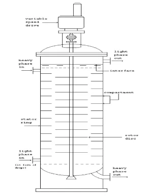
The RDC column is a mechanical device that is widely being used in the study of liquid-liquid extraction. In this column, the process of the extraction is brought about by dis-persing one of the liquid phase into the other, the continuous phase. The counter current flow of the dispersed liquid, the drop phase, in the column is affected by the difference in densities of the two liquids. As the drops flow up the column, drops may break into smaller drops as they hit the rotating discs located along the column.
Several models have been developed for processes involving RDC columns. These models show that the hydrodynamic and the mass transfer processes are important factors for the column performance ([10],[2],[1]).
Even though the mathematical models for simulating the column have been developed successfully, the production of simulation data for further analysis is time consuming. There-fore, an alternative approach based on Artificial Neural network is considered to assist in speeding up the simulation process.
In this paper, we introduced a new application of Neural Network technique in modelling the extraction processes involved in the RDC column.
2
Rotating Disc Contactor Column
The rotating disc contactor column is one of the agitated mechanical devices that is widely being used in the study of liquid-liquid extraction. It was initially developed in the Royal Dutch/Shell laboratories in Amsterdam by Reman in 1948-52. Some hundreds of RDCs are at present in use world-wide, ranging from less than 1m to 4.5m in diameter (Koster[5]).
stator ring opening, compartment height, number of compartments and disc rotational speed [4]. Careful consideration must be given to these parameters in designing a satisfactory and efficient RDC column.
In the RDC column, the mechanism of mass transfer across an interface between two liquid phases is based on penetration theory. This theory was proposed by Higbie in 1935[3], which assumed that a packet of fluid with bulk concentration, travel to the interface at a distance, from its original position. At the interface the fluid packets undergo molecular diffusion for a short exposure of time, before being replaced by another fluid packet. When the drop is dispersed into the column, we assumed that the drop has an initial uniform concentration and as well as the concentration of the medium phase. The amount of solute transferred to the drop can be obtained by using the concept of diffusion in a sphere (see [7]). Since in the RDC column, the interface of the drops in contact with the medium is spherical, the driving force from the drop surface to the bulk concentration in the drop is considered to be the quadratic driving force.
2.1
Process of Mass Transfer Based on Quadratic Driving Force
The mass transfer model based on quadratic driving force is used if one of the interface of the two liquid in contact is spherical. The mass transfer across the surface of the sphere given by flux J is define as
J = 2Dyπ
2
6d (
(c0−c1)2−(Cav−c1)2
Cav−c1
), (1)
whereCav is the average concentration of the drop at timetandc1andc0are the initial and
boundary concentrations respectively. Dy is the molecular diffusivity in the drop phase,y.
dis the diameter of the drop. ((c0−c1)2−(Cav−c1)2
Cav−c1 ) is known as the quadratic driving force. Meanwhile the flux transfer in the continuous phase is given by
J =kx(cb−cs), (2)
where cb and cs are the bulk concentration in continuous phase and the concentration at
the interface respectively. kx is the film mass transfer coefficient of the continuous phase,
x. At the interface, (1) and (2) are equal, that is 2Dyπ2
6d (
(c0−c1)2−(Cav−c1)2
Cav−c1
) =kx(cb−cs). (3)
According to Slater(1985), fractional approach to equilibrium is used to relate analytical results to a mass transfer coefficient that is
F =Cav−c1
c0−c1
. (4)
Substituting (4) into (3), we get
2Dyπ2
6d (ys−y0)
1−F(t)2
F(t)
=kx(xb−xs). (5)
Now, let consider the situation at the drop surface. Equilibrium between the medium and the concentration of drop is governed by equation
ys=f(xs), (6)
where f(xs) = xs1.85. The drop and medium concentration,ys and xs, at the surface are
found by solving non-linear equations of (6) and (5). Then the average concentration of the drops can be obtained by equation
yav−y0
ys−y0
=F(t). (7)
In this work, we assume that each compartment in the RDC column has ten different classes which will place ten different sizes of the drops. We are also interested to find the mass transfer of multiple drops of 10 different drop sizes. In order to get the total average concentration of the drops in one compartment,Yav we use
Yav =
PN cl
i=1ni×Vdrop,i×yav,i
PN cl
i=1ni×Vdrop,i
(8)
where N clthe number of different class, Vdrop,i the volume of the drop with sizei andni
is the number of drop.
Then the amount of mass transfer of the drops can be obtained by applying mass balance equation, that is
Fx(xin−xout) =Fy(yout−yin), (9)
where Fx and Fy are the flow rate of continuous and the drop phase respectively. The
concentrationxin andyinare the uniform initial concentration of the continuous and drop
phase. xout andyoutare the exiting concentration of the continuous and drop phase. In the
RDC column, we assume Yav is the exiting concentration of the drop at first compartment
and also this concentration is assumed to be the initial concentration of the drop in the next compartment.
The simulation based on this model was done by Talib[10] and Arshad[1]. This mathe-matical model is used successfully to simulate the column. But the production of simulation data for further analysis is time consuming. Therefore, an alternative approach based on Artificial Neural Network is considered to assist in speeding up the simulation process.
3
The Artificial Neural Network (ANN) Model
In this work, the simulated data from the literature (Arshad[1]) was used. In practice, any size set of training data can be generated. However, the larger the training data set, the better the performance.
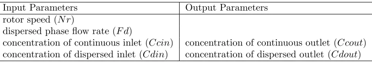
In the process of modelling an RDC column, the input and output parameters are shown in Table 1.
Table 1: Input and output parameters of the system.
Input Parameters Output Parameters rotor speed (N r)
dispersed phase flow rate (F d)
concentration of continuous inlet (Ccin) concentration of continuous outlet (Ccout) concentration of dispersed inlet (Cdin) concentration of dispersed outlet (Cdout)
There ia a set of 256 data available and this data set consists of four columns of input data and two column of output data. It is divided into two sets, that are training set and validating set. To increase the numerical stability of the training, the data are normalized by taking the maximum value for each parameter and then divide each entry in parameter by the corresponding maximum value respectively.
Here, a network with two layers of neurons is considered. The first layer, the input layer is a pre-processing layer that simply distributes the inputs to the next layer. Bias or reference is added at each layer except at the output layer.
The data from the input neurons is propagated through the network via the intercon-nections. Every neuron in a layer is connected to every neuron in adjacent layers. A scalar weight is associated with each interconnection.
Neurons in the hidden layers receive weighted inputs from each of the neurons in the previous layer and they sum the weighted inputs to the neuron and then pass the result-ing summation through a non-linear activation function. In this study the Log-Sigmoidal activation function is used.
The weighted sum to thekth neuron in thejth layer,Skj, wherej≥2 is given by
Skj =
NXj−1
i=1
(Wi,kj Iij−1) +bjk, (10)
where Iij−1 is the information from theith neuron inj-1th layer,bj,k is the bias term and
Nj−1 is the number of neurons in the previous layer (j-1). In this casej=2 and also the
coefficient of the bias is 1. When j= 1 (10) becomes
Skj=
Np
X
i=1
(Wi,kj pi) +bjk, (11)
where pi is the information of the input parameter andNp is the number of neurons or the
number of input parameters.
Ojk=fj(Skj), (12) where fj is the activation function used in thejth layer.
The following section will describe the method used to choose the best architecture of the network and the algorithm used to train the neural net.
3.1
MLP Network Training
There are different methods for finding the optimized network structure and among them are network pruning algorithm and network growth algorithm [6]. The pruning Neural Net-works assume that a neural network with superfluous parameters has been trained already. Therefore, pruning is the technique of removing between neurons in two connected layers, which are superfluous for solving the problem. The growth approach, which corresponds to constructive procedure, start with a small network and then it adds additional hidden neuron and weights, until a satisfactory solution is found. In this work we used the later technique to find the best optimal structure of the Network.
Here, the feed forward multi-layers perceptron (MLP) using Back-propagation algorithm was selected for training the data. In this case, the Levenberg-Marquardt algorithm was used to determine how to adjust the weights to minimize performance. The algorithm is a variation of Newton’s method that was designed for minimizing function that are sums of squares of other nonlinear function [8]. This is very well suited to neural network training where the performance index is the mean squared error.
The errors (F) between networks output (O) and the targets (T) are summed over the entire data set and updating of the weight is performed after every presentation of the complete data set.
F =
Q
X
q=1
(Tq−Oq)T(Tq−Oq) (13)
where Qis the number of examples in the data set.
To identify the process model, first of all the neural network has been trained. The training process of the data is performed in two steps. At beginning, the weights and biases are initialized before training with data from the training set. This data is used to calculate the error F and to update the weights and biases. Then all the weight and bias obtained are used to validate the second set of data.
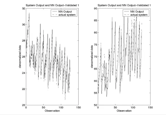
The comparison between NN outputs and MM outputs are made by plotting the graphs, as shown in Figure 1.
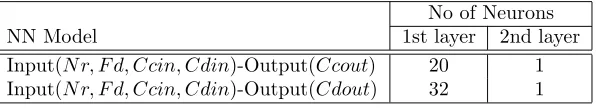
Table 2: Number of neurons in each layer for the NN Model.
No of Neurons
NN Model 1st layer 2nd layer
Figure 1: Simulated data ofCCout from NN Model and MM Model
4
Result And Conclusion
The system which describe the process of mass transfer in the RDC column is a multi-input-multi-output (MIMO) system. Since MIMO system can always be separated into group of multi-input-single-output (MISO) system, here we consider two MISO system for accessing a Neural Network Model. The inputs and the outputs of the first MISO system are represented by N r, F d, Ccin, Cdin and Ccout respectively. Meanwhile for the second system, the inputs and the output areN r, F d, Ccin, Cdin andCdout.
In this study, the NN models with two hidden layers architecture are suitable for mod-elling the RDC column with four inputs and one output. The number of neurons for each layer in respective model are summarized as shown in Table 2.
The Neural Network Model can be written as
am=fm2(W
2
mf
1
m(W
1
mp+b
1
m) +b
2
m (14)
whereamindicates the output ofm-th MISO system. In this casem= 1,2. Both models use
Log-Sigmoid at first layer and Linear functions at second layer as their activation functions. W1mandW2mis the weight matrix at the first and second layer, respectively. b1mandb2mis the bias matrix at first and second layer, respectively. pis the information about the input parameters. These matrices are given in the Appendix 2 and 3.
References
[1] Arshad, K.A., Parameter Analysis For Liquid-Liquid Extraction Coloumn Design, Ph.D. thesis, Bradford University, Bradford, U.K., 2000.
[2] Ghalehchian, J. S. ,Evaluation of Liquid-Liquid Extraction Column Performance for Two Chemical System, Ph.D. thesis, Bradford University, Bradford, U.K., 1996.
[3] Godfrey J.C., Slater, M. J.,Liquid-Liquid Extraction Equipment, John Wiley & Sons, 1994.
[4] Korchinsky, W.J.,Liquid-Liquid Extraction Equipment, J. Wiley and Sons, 1994.
[5] Koster, W.C.G.,Handbook of Solvent Extraction, J. Wiley and Sons, 1983.
[6] Liqun Ren, Zhiye ZhaoAn Optimal Neural Network and Concrere strength modeling, Advance in Engineering Software, 2002, 33 117-130.
[7] Maan. N., et. al., Mass Transfer Model of A Single Drop in The RDC Column, Sim-posium Kebangsaan Sains Matematik ke-10, 2002, 10 217-227.
[8] Martin,T.H., Howard,B.D., et. al.Neural Network Design, PWS Publishing Company, Boston, 1995.
[9] Nikola, K.K.,Foundations of Neural Networks, Fuzzy System and Knowledge Engineer-ing, The MIT Press, Cambridge, 1996.
APPENDIX 1 (The Schematic Diagram of RDC Column.)
APPENDIX 2 (The weights and biases for the first Neural Network Model )
W1
1 is the weights obtained after the training process for the neurons at the first layer of
the first NN model. The number of epochs in this training is 200.
W11=
−11.6016 −11.4513 −23.8213 −31.5770 9.0296 7.5653 21.5436 −9.4145
−17.5673 −29.0583 11.2306 −10.9766
−20.4849 33.5341 −26.3973 6.0839
−15.6670 8.5482 −4.0108 −8.2985 0.4737 5.7461 0.2600 −0.3223 16.2065 7.8363 8.2652 2.2816
2.0333 −2.7433 −13.6795 27.8708
−9.9680 −7.8010 −11.0229 −18.0821 0.6244 3.2629 −62.6489 0.3498 4.4232 0.1250 −45.6448 −5.0224 1.0026 3.2382 −2.1442 0.0144 3.9003 −1.7057 −51.7997 −16.4801 2.3319 2.3188 −25.6531 20.4013 48.4936 27.1190 7.8771 2.5081
−11.6195 −9.5550 −22.8164 4.3291 12.3347 −1.8299 −62.4832 −4.9297
−7.3174 7.7746 7.3071 −1.9144
−3.7421 −1.6861 9.2493 −9.3748
W2
1 is the weights for the neurons at the second layer of the first NN model. b11 andb21are
the biases at the first and second layer for the first NN model respectively. These matrices are obtained after the training process is completed.
(W12)T =
−0.0220
−0.0241
−0.0286
−0.0234
−0.0268 0.5355
−0.0315 0.1221
−0.0092
−0.0219
−0.0290
−0.0313
−0.9652
−0.0164
−0.0360
−0.0519 0.0400
−0.0255 0.0963
−0.1150
, b11=
70.8487
−28.3991 43.4188 30.3637 19.5125
−2.7230
−30.4527 6.5653
−54.7637 37.7691 49.0575 40.9930 0.3538 51.6082
9.7691
−50.2908 31.1412 56.7379
−7.4703 0.2141
APPENDIX 3 (The weights and biases for the second Neural Network Model )
W1
2 is the weights obtained after the training process for the neurons at the first layer of
the second NN model. The number of epochs in this training is 27.
W21=
22.2592 −2.3857 34.5208 3.0593
−12.4202 6.0073 23.7224 −0.9487 12.7946 −2.0977 −22.9816 −24.5593
−4.5848 −3.8284 −24.7882 23.7924 28.2238 6.5186 −18.2248 −1.3169 30.3659 4.6801 11.2100 −4.9670
−3.5905 −12.3052 41.7379 −4.9146
−29.8498 2.9648 −23.7783 −5.6348 24.6017 6.9954 28.6317 −0.0723
−3.7565 −16.1316 5.5048 −8.0170 19.5502 7.2762 −38.9506 4.9633 16.0570 −1.0472 28.6320 18.0387 29.6545 10.2237 1.3754 4.1443 25.3792 4.2255 −13.6677 14.4606
−24.1300 4.4447 17.9407 −10.1784
−16.9272 −5.1056 39.6359 −15.0054 27.3130 −5.2066 30.4466 12.7114 17.2434 −2.0261 43.9374 1.2715
−10.4822 −24.6501 5.9526 −1.6809 26.0817 3.4881 40.3425 1.1963
−26.2033 −6.2866 −31.5111 7.4570
−8.7330 −0.1954 48.8809 −14.5085 23.6011 −11.5882 −28.6434 2.7058
−17.4144 1.1948 −24.0002 −18.3442
−24.4872 −5.0249 44.9292 −1.0773
−17.9365 11.9954 28.0205 −7.3979
−11.2146 5.6222 −32.5146 10.4748 8.2554 3.4497 −51.3152 −11.7470
−9.6670 −3.2912 45.2276 9.6988
−20.7008 8.9834 −25.3425 18.0730
−20.2701 7.0565 −20.2580 18.7095 25.5094 2.8199 22.5681 13.9088
W2
2 is the weights for the neurons at the second layer of the second NN model. b12 andb22
are the biases at the first and second layer for the second NN model respectively. These matrices are obtained after the training process is completed.
(W22)T =
0.0600 0.1424
−0.0085
−0.0145
−0.0417 0.0443 0.0442
−0.0104 0.0367
−0.0097
−0.0619 0.0572
−0.0346 0.0226 0.0480
−0.0252 0.0214 0.0112 0.0267 0.0490
−0.0452
−0.0248
−0.0106
−0.0445 0.0410 0.0105 0.0845
−0.2278
−0.2626
−0.1197 0.0753 0.0899
, b12=
−55.8841
−6.3854 23.0315 13.1581
−17.3058
−38.4585
−17.3068 49.3995
−54.1203 18.5119
9.9117
−54.5353
−38.2227
−26.4513 10.5744
−6.6788
−51.1818
−54.6847 16.6197
−58.9224 43.0477
−27.7743 15.6928 46.5654
−21.3536
−14.1058 22.0037 52.5239
−44.0466 13.2290
9.1784
−45.3529