A Zero-Sum Electromagnetic Evader-Interrogator
Differential Game with Uncertainty
H.T. Banks and Shuhua Hu
Center for Research in Scientific Computation North Carolina State University
Raleigh, NC 27695-8212
In Memoriam of Prof. L. D. Berkovitz
February 21, 2011
Abstract
We consider dynamic electromagnetic evasion-interrogation games in which the evader can use ferroelectric material coatings to attempt to avoid detection while the interrogator can manipulate the interrogating frequencies to enhance detection. The resulting problem is formulated as a two-player zero-sum dynamic differential game in which the cost functional is based on the expected value of the intensity of the reflected signal. We show that there exists a saddle point for the relaxed form of this dynamic differential game in which the relaxed controls appear bilinearly in the dynamics gov-erned by a partial differential equation. We also present a computational framework for construction of approximate saddle point strategies in feedback form for a special case of this relaxed differential game with strategies and payoff in the sense of Berkovitz.
AMS subject classifications: 83C50, 91A23, 49N70, 49N90, 65M32, 68T37, 60J70.
1
Introduction
In an electromagnetic evasion-interrogation game, the evader wishes to minimize the in-tensity of the reflected signal to remain undetected in carrying out his mission while the interrogator wishes to maximize the intensity of the reflected signal to detect the attacker. The results in [5] demonstrated that it is possible to design ferroelectric/ferromagnetic ma-terials with appropriate dielectric permittivity and magnetic permeability to significantly attenuate reflections of known electromagnetic interrogation signals from highly conductive targets such as airfoils and missiles. However the results in [6] showed that if the evader employed a counter interrogation design based on a fixed set of known interrogating frequen-cies, then by a rather simple counter-counter interrogation strategy (use of an interrogating frequency little more than 10% different from the assumed evader design frequencies), the interrogator can easily defeat the evader’s material coatings counter interrogation strategy to obtain strong reflected signals. Thus, one can readily conclude from these two results that the evader and the interrogator must each try to confuse the other by introducing significant uncertainty in their design and interrogating strategies, respectively.
Based on this consideration, a static electromagnetic evasion-interrogation game (in the spirit of mixed strategies introduced by von Neumann [37]) was considered in [2], where the problem is mathematically formulated as a minimax game over sets of probability measures taken with the Prohorov metric. In this case this is equivalent to the weak star topology for the set of probability measures considered as a subset of the dual C∗ of C, the bounded continuous functions with the supremum norm. In this formulation, the evader does not choose a single coating, but rather has a set of possibilities available for choice and only chooses the probabilities with which he will employ the materials on a target. By choosing his coatings randomly (according to a best strategy to be determined in a minimax game), he prevents adversaries from discovering which coating he will use – indeed, even he does not know which coating will be chosen for a given target. The interrogator, in a similar approach, determines best probabilities for choices of frequency and angle in the interrogating signals. Using compactness and approximation properties in the context of the Prohorov metric, the authors in [2] present a rather complete theoretical and computational framework for these static problems. A more realistic (for some scenarios) dynamic setting is initially introduced in [3] by consideration of time dynamics in the problem, wherein the evader is allowed to make dynamic changes to his strategies in response to the dynamic input information with uncertainty on the interrogator’s actions.
saddle-point strategies in feedback form for a special case of this differential game. Some summary remarks are given in Section 4.
2
Problem Formulation and Saddle Points for the
Re-laxed Differential Game
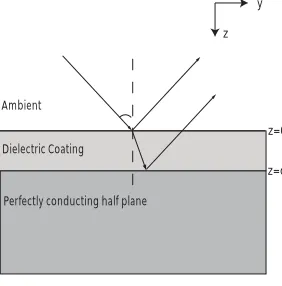
The cost functional is based on the intensity of reflected signals from an object such as an airfoil or missile coated by a radar absorbent material of constant thickness. There are several ways to treat the electromagnetic scattering [5, 6]. One fundamental approach is to employ the far field pattern for reflected waves computed directly using Maxwell’s equations. As detailed in [2], in two dimensions for a reflecting body with a given coating layer with an interrogating plane wave E(i), the scattered field E(s) satisfies the Helmholtz equation [12]. An alternative and much less computationally expensive one (as well as equally accurate in this setting – see [5, 6]) is to calculate the reflection coefficient based on a simple planar geometry (e.g., see Fig. 1) with Fresnel’s formula for a perfectly conducting half plane.
Dielectric Coating
z y
z=0
z=d
Ambient
Perfectly conducting half plane
Figure 1: Interrogating high frequency wave impinging (angle of incidence φ) on coated (thickness d) perfectly conducting surface
We will use the reflection coefficient to measure the strength of backscattering. We assume that a normally incident electromagnetic wave with the angular frequency ω is assumed to impinge the half plane. Then the corresponding wave length in the air is 2πc/ω, where the speed of light is c = 3 ×10⁸. Thus, the reflection coefficient R for a wave impinging on a coating layer of thickness d with relative dielectric permittivity and relative magnetic permeability μis given by
R(μ, , ω, d) = r1+r2
where
r1 = − √μ
+√μ and r2 = exp (2i
√
μωd/c). (2.2) This expression can be derived directly from Maxwell’s equation by considering the ratio of reflected to incident waves, for example, in the case of parallel polarized (T Ex) incident
wave (e.g., see [5, 23]).
Control of reflections by the evader is effected via local currents in a composite layered reflec-tor device that can be used to control the dielectric permittivity and magnetic permeability in a target coating layer as discussed above and in more detail in [5]. The reflector contains a ferrite layer and a ferroelectric layer as constituents. The key element of the device is that the material properties μ = μ(H) and =(E) of the composite layers are controllable in terms of the magnetic mean and the electric mean in the layers, and thus can support agile frequency attenuation. Control is implemented via local circuits which can produce rapidly changing E fields. Since the E and H fields are connected via Maxwell’s equations, if the evader controls the dielectric permittivity via these local E fields, this also produces rapid changes in the magnetic permeability μ.
For our formulation we assume that the evader “controls” dielectric permittivity of the surface coatings by choosing parameters ε = Re() from a compact admissible set E ⊂ R+ in a measurable (i.e., t → ε(t) is a measurable function) time dependent manner. (Here
R+ denotes the set of non-negative real numbers.) This produces changes in the magnetic
permeability which for our initial formulation here we assume incorporates uncertainty into the reflected signal. For simplicity, we assume the real part x of the magnetic permeability μ=x+iμi of the coating has uncertainty described by an Itˆo diffusion process Xt satisfying
the stochastic differential equation
dXt =b(Xt)dt+σ(Xt)dWt. (2.3)
HereWt denotes the standard Brownian motion and bothb=b(x) (the mean rate of change
forx=Re(μ)) andσ are non-random functions that are assumed to be Lipschitz continuous. In addition, we assume that the interrogator has control of the frequency ω of the interro-gating electromagnetic signals. At each time t ∈ [t0, T] (t0 ≥ 0), the interrogator chooses parameters ω from a compact admissible set Ω⊂R+.
2.1
Evolution of the Expected Value of Intensity of Reflected
Sig-nal and a Dynamic Differential Game
Let χ(x, ε, ω) = |R(x+iμi, ε+ii, ω, d)|, where μi and i denote the imaginary parts of μ
and , respectively, which are assumed fixed throughout this presentation. We then define ˜
v(t, x) =Ex
t
t0
λeλ(s−t0)χ(X
s, ε(s), ω(s))ds+v0(Xt)
,
where Ex[ · ] denotes the expectation with respect to the probability law of {Xt : t ≥ t0}
when its initial value is X(t0) = x, λ > 0 is a discount parameter, and v0 is a nonnegative function that is used to denote the initial (t =t0) intensity of reflected signal.
Following a standard technique for treating integrals (see Section 10.3 of [31]), we next define the Ito diffusion Yt in R2 by
dYt =d
Xt
Zt
=
b(Xt)
λeλ(t−t0)χ(X
t, ε(t), ω(t))
dt+
σ(Xt)
0
dWt.
Let g(t, x, z) = E[Zt+v0(Xt) | Y(t0) = (x, z)T], where E[ · | · ] denotes the conditional
expectation. Then we have
˜
v(t, x) =g(t, x,0). Here the generator of the Itˆo diffusion process {Yt:t≥t0} is
Lφ(x, z) =b(x) ∂
∂xφ(x, z) + 1 2σ
2(x) ∂2
∂x2φ(x, z) +λe
λ(t−t0)χ(x, ε(t), ω(t)) ∂
∂zφ(x, z). It then follows from Section 8.1 in [31] thatg satisfies the backward Kolmogorov equation
∂
∂tg =Lg, g(t0, x, z) =z+v0(x). (2.4) A discussion of the relationship between this state and the semigroup generated by L can be found in [15].
Since g = ˜v +z is the solution to (2.4), it follows that ˜v satisfies ∂
∂tv(t, x) =˜ b(x) ∂
∂x˜v(t, x) + 1 2σ
2(x) ∂2
∂x2˜v(t, x) +λe
λ(t−t0)χ(x, ε(t), ω(t)),
˜
v(t0, x) =v0(x).
Now let v(t, x) =e−λ(t−t0)v(t, x). It is easy to show that˜ v satisfies
∂
∂tv(t, x) = b(x) ∂
∂xv(t, x) + 1 2σ
2(x) ∂2
We note that the state v in this formulation is v(t, x) =Ex
t
t0
λe−λ(t−s)χ(Xs, ε(s), ω(s))ds+e−λ(t−t0)v0(Xt)
,
the expected value of a measure of the reflected intensity.
We restrict x to be in a finite interval [x,x], and set the boundary conditions to be zero.¯ Thus we will consider the state equation
∂
∂tv(t, x) =b(x) ∂
∂xv(t, x) + 1 2σ
2(x) ∂2
∂x2v(t, x)−λv(t, x) +λ χ(x, ε(t), ω(t)), v(t, x) = 0, v(t,x) = 0,¯
v(t0, x) =v0(x).
(2.5)
The objective of the game for the evader is to choose a strategy such that the intensity of the reflected signal is as small as possible while the objective for the interrogator is to choose a strategy so that the intensity of the reflected signal is as large as possible. Hence, the cost functional for a zero-sum differential game with uncertainty can be formulated by
J(ε, ω) =
T
t0 x¯
x
v(t, x;ε, ω)dxdt. (2.6)
A number of approaches have been used in the literature to study infinite-dimensional dif-ferential games. One approach is based on the theory developed by Elliott and Kalton [16] for differential games in Euclidean spaces. For example, an infinite-dimensional differential game on the infinite horizon was studied in [24] with strategies in the sense of Elliott and Kalton, and the value function of the differential game is characterized as the unique vis-cosity solution of the Hamilton-Jacobin-Isaacs equation. The other approach is based on the theory developed by Berkovitz [7] for differential games in Euclidean spaces, wherein the definition of strategy is a combination of “K strategies” discussed by Isaacs [22] and Friedman’s lower strategy (e.g., see [19, 20]) and the definition of payoff and saddle point follows that of Krasovskii and Subbotin [25]. For example, infinite-dimensional differential games with strategies and payoff in the sense of Berkovitz were studied in [21] and [35] for finite horizon and infinite horizon, respectively, and the value function is characterized as the unique viscosity solution of Hamilton-Jacobi-Isaacs equation. It should be noted that the principle result of all of these investigations is that if the so-called Isaacs condition holds then the differential game has a value. The interested readers can refer to [34] for a readable short review on the history of differential games.
For the game that we present here, the Isaacs condition does not hold as the function
x¯
x
that is used to circumvent this difficulty is to enlarge the class of controls to include relaxed controls (e.g., see [17, 32, 41]). Hence we will consider the game in a corresponding relaxed form in the remaining of this paper.
2.2
Relaxed Differential Game
The notion of relaxed control, or generalized curve, was introduced into the calculus of variations (in the 40’s) and optimal control (in the 60’s) by a number of distinguished contributors such as Young [42, 43], McShane [28, 29, 30], Filippov [18] and Warga [38, 39, 40]. Since then, it has been studied by many other researchers (e.g., see [1, 10, 11, 27]). Before we give the relaxed forms for (2.5) and (2.6), we will introduce needed theoretical background information on relaxed controls (e.g., see [17, 39, 40]). Let C(Ω) and C(E) denote the spaces of continuous functions equipped with usual supremum norm, and C∗(Ω) andC∗(E) be their corresponding topological dual spaces taken with the weak star topology which is equivalent to the Prohorov metric topology [9, 33] used in the static games in [2]. We define the spaces P(Ω) andP(E) as the spaces of all regular probability measures defined on the Borel subsets of Ω and E, respectively. Then with the Prohorov metric, P(Ω) and
P(E) are compact and convex subsets of C∗(Ω) and C∗(E), respectively. In addition, as noted above convergence in the Prohorov metric is equivalent to weak star convergence. For more information on Prohorov metric, the interested readers can refer to [9, 33].
Let L1(t0, T;C(Ω)) be the Banach space of Lebesgue integrable functions from [t0, T] to C(Ω) with the norm
gωL1(t0,T;C(Ω))=
T
t0
gω(t)C(Ω)dt.
The Banach space L1(t0, T;C(E)) and its norm is similarly defined. It is known that both L1(t0, T;C(Ω)) and L1(t0, T;C(E)) are separable. We denote the topological dual of L1(t0, T;C(Ω)) andL1(t0, T;C(E)) byL1(t0, T;C(Ω))∗ and L1(t0, T;C(E))∗, respectively. By the Dunford-Pettis theorem (e.g., see [40, Theorem IV.1.8]), we have the equivalence that
L1(t0, T;C(Ω))∗ ∼=L∞(t0, T;C∗(Ω)) and
L1(t0, T;C(E))∗ =∼L∞(t0, T;C∗(E)).
Here L∞(t0, T;C∗(Ω)) is a Banach space of essentially bounded measurable functions from [t0, T] to C∗(Ω) with the norm
ΦωL∞(t0,T;C∗(Ω)) = ess sup t∈[t0,T]
|Φω(t)|(Ω).
A sequence {Φω,j}inL∞(t0, T;C∗(Ω)) is said to be convergent in this topology if there exists
a point Φω ∈L∞(t0, T;C∗(Ω)) such that for any gω ∈L1(t0, T;C(Ω)) we have
lim
j→∞
T
t0
Ω
gω(t, ω)Φω,j(t)(dω)dt=
T
t0
Ω
gω(t, ω)Φω(t)(dω)dt.
The convergence of a sequence in L∞(t0, T;C∗(E)) with the weak star topology is similarly defined.
A relaxed control for the interrogator is a mapping Φω : [t0, T] →P(Ω), and this mapping
is measurable (respectively, continuous) if
Ω
hω(ω)Φω(t)(dω) is measurable (respectively,
continuous) function of t ∈ [t0, T] for every continuous real-valued function hω on Ω. A
relaxed control for the evader Φε : [t0, T] → P(E) is defined similarly. We shall identify
these controls which differ only on a set of measure zero. Let
R(Ω) ={Φω |Φω : [t0, T]→P(Ω) is measurable}.
and
R(E) ={Φε|Φε : [t0, T]→P(E) is measurable}.
LetBΩ and BE denote the unit ball of L∞(t0, T;C∗(Ω)) and L∞(t0, T;C∗(E)), respectively. That is,
BΩ ={Φ∈L∞(t0, T;C∗(Ω)) | ΦL∞(t0,T;C∗(Ω)) ≤1}
and
BE ={Φ∈L∞(t0, T;C∗(E))| ΦL∞(t0,T;C∗(E)) ≤1}.
Then the weak norm topology and weak star topology ofBΩ (respectively,BE) coincide, and with this topology BΩ (respectively,BE) is a compact metric space (see [40, Theorem I.3.11 and Theorem I.3.12]). Note that for any Φω ∈R(Ω) and Φε ∈R(E) we have Φω(t)(Ω) = 1
and Φε(t)(E) = 1. Hence, R(Ω)⊂BΩ and R(E)⊂ BE. In addition, we have the following
important results.
Theorem 2.1. (See [40, IV.2.1] or [17, Theorem 3.9]) The sets R(Ω) and R(E) can be considered as closed convex subsets of the unit ball ofL∞(t0, T;C∗(Ω)) andL∞(t0, T;C∗(E)), respectively, so with the weak star topology both R(Ω) and R(E) are compact.
Let Φω ∈ R(Ω) and Φε ∈ R(E). Then by Lemma 3.13 in [17] we know that Φε×Φω is
a measurable relaxed control on E ×Ω, and Φε ×Φω can be considered to belong to the
unit sphere of the topological dual L∞(t0, T;C∗(E ×Ω)) of L1(t0, T;C(E ×Ω)). With this background information on relaxed controls, we can now reformulate the state equation (2.5) in relaxed control form
∂
∂tv(t, x) = b(x) ∂
∂xv(t, x) + 1 2σ
2(x) ∂2
∂x2v(t, x)−λv(t, x) +f(t, x), v(t, x) = 0, v(t,x) = 0,¯
v(t0, x) =v0(x),
where
f(t, x) =λ
Ω
E
χ(x, ε, ω)Φε(t)(dε) Φω(t)(dω). (2.8)
The cost functional corresponding to the relaxed controls Φε and Φω is defined by
J(Φε,Φω) =
T
t0 x¯
x
v(t, x; Φε,Φω)dxdt. (2.9)
Hence, for this relaxed formulation (2.9) with (2.7), the evader does not choose a single coating at each time t, but rather has a set of possibilities available for choices. The inter-rogator, in a similar approach, determines best probabilities for choices of frequency in the interrogating signals at each time t.
Remark 2.2. From (2.1), it is easy to see that χ is continuous on [x,x]¯ × E × Ω. By assumption both E and Ω are compact. Hence, χ is bounded. Let
fε(t, x, ω) =
E
χ(x, ε, ω)Φε(t)(dε).
Then by the Lebesgue dominated convergence theorem we know thatfε(t,·,·)is continuous on
[x,x]¯ ×Ωfor fixedt, and by the definition of relaxed controls we knowfε(·, x, ω)is measurable
for fixed (x, ω). In addition, we have
|fε(t, x, ω)| ≤ χC([x,¯x]×E×Ω)Φε(t)(E)
= χC([x,¯x]×E×Ω).
(2.10)
Thus, fε ∈ L∞(t0, T;C([x,x]¯ ×Ω)), which implies that fε ∈ L1(t0, T;C([x,x]¯ ×Ω)). Note
that
f(t, x) =λ
Ω
fε(t, x, ω)Φω(t)(dω).
Hence, f(t,·) is continuous on [x,x]¯ for fixed t, and f(·, x) is measurable for fixed x. Simi-larly, we find
|f(t, x)| ≤λχC([x,x¯]×E×Ω). (2.11)
Thus, f ∈ L∞(t0, T;C([x,x]))¯ . In addition, by Fubini’s theorem we can exchange the order of integration in (2.8).
2.3
Existence of Saddle Points for Relaxed Differential Game
In this section we show that the relaxed form of the minmax dynamic differential game for (2.9) subject to (2.7) has a saddle point. We assume that there exists a positive constant σinf such that σ(x) ≥ σinf for any x ∈ [x,x]. Let¯ H = L2(x,x),¯ V = H01(x,x), and denote¯ the topological dual space V∗ by V∗ =H−1(x,x). If we identify¯ H with its topological dual
· H and · V and · V∗ are used to denote the norms inH, Vand V∗, respectively, ·,· denotes the inner product in H, and ·,·V∗,V represents the duality paring between V∗ and
V. Following standard conventions, we use an over dot ( ˙) to denote the derivative with respect to the time variable t, and use prime () to represent the derivative with respective to the space (i.e., permeability) variable x. In addition, for convenience we may use · ∞ to denote both the norms in L∞(x,x) and¯ C([x,x]).¯
Define the sesquilinear forma on V×V by a(φ, ψ) =−bφ, ψ+1
2φ
,(σ2ψ)+λφ, ψ. (2.12) By Remark 2.2, we know that f(t) ∈ C([x,x]). Hence, we may rewrite (3.2) in the weak¯ form
v(t), ψ˙ V∗,V+a(v(t), ψ) =f(t), ψ,
v(t0) =v0 (2.13)
for any ψ ∈ V. Here and elsewhere v(t) and f(t) denote the functions v(t,·) and f(t,·), respectively.
Theorem 2.3. Let v0 ∈ H and assume σ is Lipschitz continuous with b ∈ L∞(x,x)¯ . Then there exists a unique solution v for (2.13) with v ∈H1(t0, T;V∗)∩L2(t0, T;V). In addition, there exists a positive constant κ such that for any t∈[t0, T]
v(t)2H ≤κ
v02H+
t
t0
f(s)2V∗ds
, (2.14)
and
T
t0
v(t)2Vds ≤κ
v02H+
T
t0
f(s)2V∗ds
. (2.15)
Furthermore, we have v ∈C(t0, T;H).
Proof. Note thatV is continuously imbedded in H, and H is continuously imbedded in V∗. Hence, there exists a constant γ >0 such that
ψH ≤γψV, for anyψ ∈V, (2.16)
and
hV∗ ≤γhH, for any h∈H. (2.17)
Since σ is Lipshcitz continuous, σ ∈L∞(x,¯x). Thus, by (2.16) and (2.17) we find that for any φ, ψ∈V we have
|a(φ, ψ)| ≤ b∞φHψH+1 2σ
2
∞φHψH +σ∞σ∞φHψH+λφHψH
≤ γb∞φVψV+ 1 2σ
2
Let =γb∞+1 2σ
2
∞+γσ∞σ∞+γ2λ. Then by the above inequality we have
|a(φ, ψ)| ≤φVψV, for any φ, ψ∈V. (2.18) For any ψ ∈Vwe also obtain
a(ψ, ψ)≥
1 2σ
2 inf −2θ
ψ2V− b
2
∞+σ2∞σ2∞
4θ ψ
2
H.
Setting θ = 1 8σ
2
inf, we have
a(ψ, ψ) +αHψ2H ≥αVψ2V, (2.19)
where αV = 1 4σ
2
inf and αH = b
2
∞+σ2∞σ2∞
4θ . By Remark 2.2, we know that f ∈ L∞(t0, T;C([x,x])). Hence,¯ f ∈L2(t0, T;V∗). Thus, by Theorem 2.1 in [4] we know that for any v0 ∈H there exists a unique solution v for (2.13) with v ∈ H1(t0, T;V∗)∩L2(t0, T;V), and (2.14) and (2.15) hold for some positive constant κ. Furthermore, v ∈C(t0, T;H), and thus the initial condition in (2.13) is meaningful.
Remark 2.4. By Remark 2.2, we know that f(t) ∈ C([x,x])¯ ⊂ H. Thus, we can easily obtain from (2.11)
f(t)2H ≤κH ≡(¯x−x)λ2χ2C([x,¯x]×E×Ω). (2.20)
By (2.14), (2.15), (2.17) and (2.20) we find
v(t)2H ≤κv02H+ (T −t0)γ2κH, (2.21)
and
T
t0
v(t)2Vds ≤κv02H+ (T −t0)γ2κH. (2.22)
From (2.21)and (2.22), we see that bothv(t)2H and
T
t0
v(t)2Vds are bounded by a positive constant which is independent of the choices of Φω and Φε.
Remark 2.5. Let v(t, x) be the solution to (2.13). Then by (2.16) and (2.18) we find |v(t), ψ˙ V∗,V| = | −a(v(t), ψ) +f(t), ψ|
≤ v(t)VψV+γf(t)HψV,
which implies that
v(t)˙ V∗ = sup φV≤1
{|v(t), φ˙ V∗,V| |φ∈V}
≤ v(t)V+γf(t)H.
By (2.20) and the above equation, we obtain
Thus, by (2.22) and integrating the above equation we have
T
t0
v(t)˙ 2V∗dt≤22κv02H+ 2(T −t0)γ2κH(2κ+ 1). (2.23)
From the above equation we see that
T
t0
v(t)˙ 2V∗dt is bounded by a positive constant that is
independent of the choices of Φω and Φε.
From the definition for J defined in (2.9), to show J is separately continuous in each of its variables, it suffices to show that for given Φε ∈ R(E) and a sequence {Φω,j} ⊂ R(Ω)
converging to Φω in R(Ω) we have
lim
j→∞
T
t0 x¯
x
v(t, x; Φε,Φω,j)dxdt=
T
t0 x¯
x
v(t, x; Φε,Φω)dxdt, (2.24)
and for given Φω ∈R(Ω) and a sequence {Φε,j} ⊂R(E) converging to Φε inR(E) we have
lim
j→∞
T
t0 x¯
x
v(t, x; Φε,j,Φω)dxdt=
T
t0 x¯
x
v(t, x; Φε,Φω)dxdt. (2.25)
Actually by using (2.21), (2.22) and (2.23) and similar arguments as in [11, Lemma 2.1], we can show that (2.24) and (2.25) both hold. For convenience, we will show (2.24) in the following lemma (similar arguments can be used to establish (2.25)).
Lemma 2.6. Let Φε ∈ R(E), and assume that the sequence {Φω,j} ⊂ R(Ω) is convergent
to Φω in R(Ω). Then (2.24) holds.
Proof. For notational convenience, we let fj = f(·,·; Φε,Φω,j) and vj = v(·,·; Φε,Φω,j).
By (2.21), (2.22) and (2.23) , we know that {vj} is bounded in C(t0, T;H) and also in
L2(t0, T;V), and {v˙j} is bounded in L2(t0, T;V∗). Thus, there exists a subsequence - again
denoted by vj - such that
vj →vˆweakly in L2(t0, T;V),
˙
vj →v˙ˆweakly in L2(t0, T;V∗).
Observe thatV is also compactly imbedded in H. Hence, by Theorem 2.1 in [36] we have vj →vˆstrong in L2(t0, T;H). (2.26)
We further observe thatL2(t0, T;H) is continuously imbedded in L1(t0, T;L1(x,x)). Hence,¯ by (2.26) we know that vj is strongly convergent to ˆv inL1(t0, T;L1(x,x)), which means¯
lim
j→∞
T
t0 x¯
x
v(t, x; Φε,Φω,j)dxdt=
T
t0 x¯
x
ˆ
Thus, to complete the proof we only need to show that ˆv =v(·,·; Φε,Φω).
Letg(t, x) = η(t)ψ(x), whereψ ∈V, andη∈C1(t0, T) withη(t0) = 0 andη(T) = 0. We set v =vj in (2.13), and then multiply (2.13) by η(t) and integrate to find
T
t0
v˙j(t), ψV∗,Vη(t)dt+
T
t0
a(vj(t), ψ)η(t)dt=
T
t0
fj(t), ψη(t)dt.
Integrating by parts for the first term of the above equation, we have
−
T
t0
vj(t), ψη(t)dt˙ +
T
t0
a(vj(t), ψ)η(t)dt=
T
t0
fj(t), ψη(t)dt. (2.27)
By Fubini’s theorem, the right side of (2.27) can be written as
T
t0
fj(t), ψη(t)dt
= T t0 x¯ x λψ(x) Ω
fε(t, x, ω)Φω,j(t)(dω)
dx η(t)dt = ¯x x λψ(x) T t0 Ω
η(t)fε(t, x, ω)Φω,j(t)(dω)dt
dx.
(2.28)
By Remark 2.2, we know that fε ∈ L∞(t0, T;C([x,x]¯ ×Ω)). Since η ∈ C1(t0, T), we have
ηfε ∈ L∞(t0, T;C([x,x]¯ ×Ω)), which implies ηfε ∈ L1(t0, T;C([x,x]¯ ×Ω)). Since Φω,j is
convergent to Φω in R(Ω), letting j → ∞, passing to the limit in (2.28) and using Fubini’s
theorem we find
lim
j→∞
T
t0
fj(t), ψη(t)dt=
T
t0
f(t), ψη(t)dt.
Now we let j → ∞ and pass to the limit term by term in (2.27) to obtain
−
T
t0
v(t), ψˆ η(t)dt˙ +
T
t0
a(ˆv(t), ψ)η(t)dt=
T
t0
f(t), ψη(t)dt.
Integrating by parts for the first term in the above equation, we find
T
t0
v˙ˆ(t), ψV∗,V+a(ˆv(t), ψ)
η(t)dt=
T
t0
f(t), ψη(t)dt. (2.29)
Note that the class of η’s for which the above holds are dense inL2(t0, T). Hence, we have (2.29) holding for all η ∈ L2(t0, T). Thus, we have ˆv satisfies the first equation of (2.13). To obtain ˆv(t0) = v0, we may use the same arguments with arbitrary η ∈ C1(t0, T) with η(T) = 0 but η(t0) = 0. Therefore, by the uniqueness of the solution for (2.13) we have ˆ
v =v.
Remark 2.7. Since the example given in [17] shows that the identity mapping from R(E)×
Theorem 2.8. (See [44, Corollary 3.2]) Let X be a nonempty compact and convex subset of a Hausdorff topological vector space, and let Y be a nonempty convex subset of a Hausdorff topological space, respectively. Suppose that J : X×Y → R satisfies (i) for each fixed
x ∈ X, y −→ J(x, y) is lower semicontinuous and quasiconvex; (ii) for each fixed y ∈ Y,
x−→J(x, y) is upper semicontinuouos and quasiconcave. Then we have
max
x∈X miny∈Y J(x, y) = miny∈Y maxx∈X J(x, y).
Moreover, if Y is compact, then J has a saddle point in X×Y.
Note that J of (2.9) is continuous and linear in each variable. Thus, by Theorems 2.1 and 2.8 we find that J has a saddle point, which is summarized in the following theorem.
Theorem 2.9. There exists a pair of relaxed controls Φ∗ω ∈R(Ω) and Φ∗ε ∈R(E) such that J(Φ∗ε,Φω)≤ J(Φ∗ε,Φ∗ω)≤ J(Φε,Φ∗ω)
for any Φε ∈R(E) and Φω ∈R(Ω).
From Remark 2.7, we have that the cost functional J is not jointly continuous, which implies that there are challenges in carrying out standard numerical approximations (such as the delta approximation or spline approximation employed in [2] for the static case and the discretization method used in [11] for computation of relaxed optimal control) in the domainR(E)×R(Ω). To circumvent these difficulties, we will consider a special case of our relaxed differential game in the remainder of this paper, where we assume that both evader and interrogator have only finite number of choices at each time t. Then we develop a computational framework to obtain approximate optimal strategies for the resulting relaxed differential game.
3
Construction of Approximate Saddle Point
Strate-gies for a Simplified Relaxed Differential Game
In this section, we assume Ω = {ω1∗, ω∗2, . . . , ω∗m} ⊂R+, and E ={ε∗1, ε∗2, . . . , ε∗l} ⊂R+, and restrict our controls to measures of the form
Φω(t) = m
j=1
uω,j(t)Δω∗j, Φε(t) = l
i=1
uε,i(t)Δε∗i, (3.1)
We consider the resulting relaxed differential game (which will be termed assimplified relaxed differential game in the remainder of this paper) with strategies and payoff in the sense of Berkovitz [7]. Specifically, in Section 3.1 we show that this game has a value and the value function is the unique viscosity solution of Hamilton-Jacobi-Isaacs equation. In Section 3.2 we employ Galerkin approximation techniques to reduce the problem into one in a finite di-mensional space, and show that these approximate differential games have a value. Moreover the corresponding value functions converge pointwise to the value function of this simplified relaxed differential game. Then in Section 3.3 we use Berkovitz’s method to construct opti-mal strategies for the approximate differential games, and show that these optiopti-mal strategies are the approximate optimal strategies for this simplified relaxed differential game.
First we introduce some necessary notation. Let uε,i : [t0, T] → R and uω,j : [t0, T] →
R be measurable nonnegative functions, i = 1,2, . . . , l and j = 1,2, . . . , m, which satisfy
l
i=1
uε,i(t) = 1 and m
j=1
uω,j(t) = 1. Let
uε= (uε,1, uε,2, . . . , uε,l)T, and uω = (uω,1, uω,2, . . . , uω,l)T.
Then we have
uε ∈ Uε[t0, T], uω ∈ Uω[t0, T],
where for t0 ≤s1 < s2 ≤T
Uε[s1, s2] ={u|u : [s1, s2]→Ul is measurable},
Uω[s1, s2] ={u|u: [s1, s2]→Um is measurable}.
Here for k ∈N we define
Uk =
μ= (μ1, μ2, . . . , μk)T ∈Rk : k
i=1
μi = 1, μi ≥0
.
Hence, both Ul and Um are convex and compact. For notational simplicity, we shall write
Uε for Uε[t0, T] and Uω for Uω[t0, T].
The corresponding relaxed control form of the state equation (2.5) is then given by ∂
∂tv(t, x) =b(x) ∂
∂xv(t, x) + 1 2σ
2(x) ∂2
∂x2v(t, x)−λv(t, x) + ˜f(x, uε(t), uω(t)), v(t, x) = 0, v(t,x) = 0,¯
v(t0, x) =v0(x).
(3.2)
Here the function ˜f : [x,x]¯ ×Ul×Um → Ris defined by
˜
f(x, με, μω) =λ m
j=1 l
i=1
μω,jμε,iχ(x, ε∗i, ωj∗) =λμ T
where B(x) is a l × m matrix with its (i, j)th element being χ(x, ε∗i, ωj∗). Observe that χ(·, ε∗i, ωj∗) is continuous in [x,x]. Hence, ˜¯ f(·, με, μω) ∈ C([x,x])¯ ⊂ H and ˜f is bounded in
the domain [x,x]¯ ×Ul×Um. In the following, we denote ˜f(·, με, μω) by F(με, μω) for ease
in presentation. It is easily seen that F :Ul×Um →H is continuous.
3.1
Value of Differential Game
In this section, we will study our differential game with strategies and payoff in the sense of Berkovitz. Specifically we will use some of the results in [21, 35] to show that our differential game has a value and this value function is the unique viscosity solution of Hamilton-Jacobin-Isaacs equation.
Define the linear operator A : V → V∗ by a(φ, ψ) = −Aφ, ψV∗,V, where a is defined in
(2.12). Then (3.2) can be rewritten in the following abstract (in V∗) form ˙
v(t) =Av(t) +F(uε(t), uω(t)), v(t0) =v0. (3.3)
and its corresponding weak form is given by
v(t), ψ˙ V∗,V+a(v(t), ψ) =F(uε(t), uω(t)), ψ, for any ψ ∈V
v(t0) =v0.
(3.4)
By (2.18), (2.19) and the arguments in [4, Section 2], we know thatA generates an analytic semigroup S(t) on H, V and V∗. Note that V is compactly embedded in H. Hence, S(t) on
H is compact (see [14, page 394]). In addition, by Theorem 2.1 in [4], we know that for any given v0 ∈ H there exists a unique solution v for (3.4) with v ∈H1(t0, T;V∗)∩L2(t0, T;V) given by
v(t) =S(t)v0+
t
t0
S(t−s)F(uε(s), uω(s))ds, (3.5)
and there exists some positive constant κ such that
v(t)2H ≤κ
v02H+
t
t0
F(uε(s), uω(s))2V∗ds
, t ∈[t0, T]. (3.6)
Furthermore, we have v ∈C(t0, T;H).
Let G : H → R defined by G(φ) =
x¯
x
φ(x)dx for any φ ∈ H. Note that H is continuously embedded in L1(x,x). Hence, for any¯ φ, ψ∈Hthere exists a positive constant κg such that
|G(φ)− G(ψ)|=
x¯
x
Now we adjoin the differential equation ˙
v0(t;t0, v0, uε, uω) =G(v(t, x;t0, v0, uε, uω)), v0(t0) = 0 (3.7)
to (3.4). Note that ˜f is bounded in the domain [x,x]¯ ×Ul×Um andF(με, μω)∈H. Hence,
by (3.6) we know that there exists some positive constant κ0 (independent of the choices of uε and uω) such that
|v0(t;t0, v0, uε, uω)|2 ≤κ0(v02H+ (T −t0)) (3.8)
for any t∈[t0, T].
We now define the strategy for evader and interrogator in the sense of Berkovitz (e.g. see [21, 34]). A strategy Γε for the evader is a choice of a sequence Πε ={πεn} of partitions of
[t0, T] and a choice of a sequence of maps ΓΠε
ε ={ΓΠε ,n
ε }, where ΓΠε ,n
ε is described below. For
notational simplicity, we will suppress the dependence on Πεin the notation and write Γε for
ΓΠε
ε and Γnε for ΓΠεε,n. Let the partition points of πεn be t0 =tεnε,0 < tεnε,1 < . . . < tnεε,nε =T
with πεn = max
1≤i≤n{t nε,i ε −t
nε,i−1
ε } → 0 as n → ∞. Each map Γ n
ε is a collection of maps
{Γn,jε }nε
j=1, where Γ n,1
ε ∈ Uε[t0, tεnε,1) and for 2≤j ≤nε,
Γεn,j :Uε[t0, tεnε,j−1)× Uω[t0, tnεε,j−1)→ Uε[tnεε,j−1, t nε,j ε ).
A strategy Γω for the interrogator is similarly defined (by replacing the subscript εtoω, and
subscript ω toε).
Note that a pair (Γnε,Γnω) ofnth stage strategies determine uniquely a pair (unε, unω)∈ Uε×Uω
as follows. Let πn = {t0 = tn,ˆ0 < tn,ˆ1 < . . . < tn,ˆnˆ = T} be the common refinement of πεn and πnω. The control functions unε = (uεn,1, un,ε2, . . . , un,εnˆ) and unω = (un,ω1, un,ω2, . . . , un,ωnˆ), where un,jε ∈ Uε[tˆn,j−1, tn,jˆ ) and un,jω ∈ Uω[tn,jˆ −1, tn,jˆ ), j = 1,2, . . . ,n. Letˆ unε,j and u
n ω,j be
the restriction of unε and unω to [t0, tn,jˆ ), respectively. On [tn,ˆ0, tn,ˆ1), we set un,ε1 = Γn,ε1 and un,ω1 = Γn,ω1. Let 1 ≤ j ≤ nˆ−1. If there exists 1 ≤ i ≤ nε such that tˆn,j = tnεε,i, then on
[tn,jˆ , tn,jˆ +1) we set uεn,j+1 = Γn,iε +1(unε,j, uω,jn ) and un,jω +1 = Γn,lω +1(unε,j, unω,j), where l is the
greatest integer such that tnω,l
ω <=tˆ n,j
and j is the integer such that tnω,l ω = tˆ
n,j
. If there exists 1≤k ≤nω such thattn,jˆ =tnωω,k, then on [tˆ
n,j, tn,jˆ +1) we setun,j+1 ε = Γ
n,l+1 ε (u
n ε,j, u
n ω,j)
and un,jω +1 = Γn,kω +1(uε,jn , unω,j), where l is the greatest integer such that tnε,l
ε <= tˆ
n,j and j
is the integer such that tnε,l ε =tˆ
n,j. The pair (un ε, u
n
ω) determined this way is called the nth
stage outcome of the pair (Γnε,Γnω) ofnth stage strategies.
Now let {v0,n} be a sequence converging to v0. For each n, we have the nth stage trajectory
¯
v(· ;t0, v0,n, unε, u n
ω) = (v0(· ;t0, v0,n, unε, u n
ω), v(· ;t0, v0,n, unε, u n ω))
T, which is the unique
solu-tion to (3.7) and (3.4) corresponding to the control funcsolu-tions unε andunω and initial condition (0, v0,n)T. Note that S(t) onHis compact. Hence, by [21, Lemma 2.2] we have the following
result.
Lemma 3.1. Let (unε, unω) be the nth stage outcome of the pair (Γnε,Γnω) of strategies on
[t0, T], and {v0,n} be a sequence converging to v0. Then the sequence {v(· ;t0, v0,n, unε, unω)}
With Lemma 3.1 and inequality (3.8), we now can define the concept of motion in the game. Any uniform limit of a subsequence of the nth stage trajectories {v(¯ · ;t0, v0,n, unε, u
n ω)}∞n=1,
where v0,n → v0, and (unε, u n
ω) is the outcome of the pair (Γ n ε,Γ
n
ω), is called the motion of
the game corresponding to strategies Γε={Γnε}and Γω ={Γnω}that starts from initial point
(t0, v0). This motion is denoted by ¯v[·;t0, v0,Γε,Γω] = (v0[·;t0, v0,Γε,Γω], v[·;t0, v0,Γε,Γω])T.
The set of all motions ¯v[· ;t0, v0,Γε,Γω] corresponding to the pair (Γε,Γω) is denoted by
V[·;t0, v0,Γε,Γω]. Similarly, we useV0[·;t0, v0,Γε,Γω] andV[·;t0, v0,Γε,Γω] denote the set
of v0[·;t0, v0,Γε,Γω] and v[·;t0, v0,Γε,Γω], respectively.
If the initial point of the augmented component of the trajectory is given by a nonnegative number v00, then the corresponding extended trajectory with controls uε and uω is denoted
by
¯
v(·;t0,¯v0, uε, uω) = [v00+v0(·;t0, v0, uε, uω), v(·;t0, v0, uε, uω)]T,
where ¯v0 = [v00, v0]T.
To complete the description of the game, we need to define the payoff structure. The payoff corresponding to a pair of strategies (Γε,Γω) is set valued and is defined by
J(Γε,Γω;t0, v0) =V0[T;t0, v0,Γε,Γω].
The evader tries to choose Γε so as to minimize all elements of J(Γε,Γω;t0, v0) and the
interrogator tries to choose Γω so as to maximize J(Γε,Γω;t0, v0). Hence, we see that the
payoff is not required to be evaluated along a trajectory of the system. We define
J−(t
0, v0) = sup Γω
inf
Γ J
(Γε,Γω;t0, v0), J+(t0, v0) = inf
Γ
sup
Γω
J(Γε,Γω;t0, v0).
(If {Qβ} is a collection of subsets of R, then sup β
Qβ sup∪βQβ and inf
β Qβ inf∪βQβ.)
Then it is easy to see that J−(t0, v0) ≤ J+(t0, v0). If J−(t0, v0) = J+(t0, v0), we denote this common value by J∗(t0, v0) and say that the game has a value equal to J∗(t0, v0). LetQ and ˜Q be two sets of real numbers. We say that Q≥Q˜ if for every q∈Q and every ˜
q ∈ Q˜ the inequality q ≥ q˜holds. Also, if α is a real number and Q is a set, by α ≥ Q we mean that α≥q for all q∈Q. A similar meaning holds forα≤Q.
A pair of strategies (Γ∗ε,Γ∗ω) is said to be thesaddle point (oroptimal strategies) for the game with the initial point (t0, v0) if the inequality
J(Γ∗ε,Γω;t0, v0)≤ J(Γ∗ε,Γω∗;t0, v0)≤ J(Γε,Γ∗ω;t0, v0)
holds for all (Γε,Γω). Note that, if (Γ∗ε,Γ∗ω) is a saddle point, then J(Γ∗ε,Γ∗ω;t0, v0) is a
singleton and is given by
We now consider games, trajectories and motions with varying initial points (τ, ϕ)∈[t0, T]×
H. Givenφ ∈H and ϕ∈H, we define
H(με, μω;ϕ, φ) =φ,F(με, μω)+G(ϕ), με∈Ul, μω ∈Um.
Observe that for any φ, ϕ ∈ H, H is continuous and linear in each variable. Since Ul and Um are both compact and convex, we have H−(ϕ, φ) =H+(ϕ, φ) for any φ, ϕ∈H, where
H−(ϕ, φ) = max
μω∈Umμminε∈UlH
(με, μω;ϕ, φ), H+(ϕ, φ) = min με∈Ul
max
μω∈UmH(με, μω;ϕ, φ).
With this equality we say that Isaacs condition is satisfied. Let H∗ =H− = H+. Then by [21, Theorem 3.2] we have that the differential game has a value J∗ = J− =J+ and it is the unique viscosity solution of the Hamilton-Jacobi-Isaacs (HJI) equation
J∗
τ +Aϕ, DJ∗+H∗(ϕ, DJ∗) = 0, (τ, ϕ)∈(t0, T)×H
J∗(T, ϕ) = 0 (3.9)
in the sense of Crandall-Lions [13]. Here DJ∗ denotes the Fr´echet differential of J∗ with respect to ϕ∈H.
In [21, 35], Berkovitz’s approach of constructing optimal strategies [7] was shown to be ap-plicable to the infinite-dimensional differential game as well. It should be noted that the Berkovitz method involves using some feedback maps to construct the saddle point for the game, where these feedback maps are obtained by using some appropriate level sets related to the value function. Hence, to use this method one needs to compute the value function
J∗ for (3.9), which is a partial differential equation in an infinite-dimensional space with the unbounded operator A involved. To overcome some of these difficulties, the authors in [34] first approximate the unbounded operator by a bounded operator (e.g., the Yosida approximation), and then study the associated approximate differential games with these bounded operators and obtain their value functions. In addition, the authors showed that the value function for the original differential game is the limit of the value functions of these approximate differential games, and the saddle point for the approximate differential game is an approximate saddle point for the original differential game. Although this method makes the problem conceptually easier, one still needs to solve a partial differential equation defined in an infinite-dimensional space. In the remainder of this paper, we address this issue by employing Galerkin approximation techniques to reduce the problem to one in a finite dimensional space. This approximation technique has been used in [4] to establish a compu-tationally feasible approximation theory for linear quadratic regulator control problems for infinite dimensional systems with unbounded input operators.
3.2
Value of Approximate Differential Game
approximate differential games indeed have values, and these value functions converge point-wise to the original value function J∗.
Let VN be a sequence of finite-dimensional subspaces of V ⊂ H. We assume the following standard [4, Sec. 4] approximation condition
(H1) For anyφ∈V, there exists a sequenceφN inVN such thatφN−φV →0 asN → ∞.
Define the operatorAN :VN →VN (which approximates A) by restriction ofa toVN×VN; this yields
−ANφ, ψ=a(φ, ψ), for all φ, ψ∈VN.
Let the operator PN denote the usual orthogonal projection of H onto VN. That is, for φ∈H, we have PNφ ∈VN is defined by
PNφ, ψ=φ, ψ, for all ψ ∈VN. (3.10)
It then follows from (H1) thatPNφ−φH →0 asN → ∞for anyφ ∈H. In addition, this projection operator can readily be extended to PN :V∗ →VN by replacing φ, ψin (3.10) by φ, ψV∗,V for all φ ∈ V∗. For this family of approximations, the approximate problem
corresponding to (3.3) is given by dvN(t)
dt =A
NvN(t) +FN(u
ε(t), uω(t)), vN(t0) =vN0 . (3.11)
Here vN(t) is the notation for vN(t,·), FN(uε(t), uω(t)) = PNF(uε(t), uω(t)), and vN0 =
PNv
0. Note that for any given uε and uω, F(uε(t), uω(t)) ∈ C([x,x])¯ ⊂ H. Hence, for
any ψ ∈ VN we have FN(uε(t), uω(t)), ψ = F(uε(t), uω(t)), ψ. Thus, the weak form of
(3.11), i.e., the approximate problem corresponding to (3.4), can be formulated as finding vN(t)∈VN which satisfies
dvN(t)
dt , ψ+a(v
N(t), ψ) =F(u
ε(t), uω(t)), ψ, ψ ∈VN,
vN(t0) =v0N.
(3.12)
Let GN : VN → R defined by GN(ψ) =
x¯
x
ψ(x)dx for any ψ ∈ VN. Then the approximate problem corresponding to (3.7) is given by
dv0N(t)
dt =G
N(vN(t)), v0N(t
0) = 0. (3.13)
Let {ψiN}Ni=1 be a basis of VN, ΨN = (ψ1N, ψ2N, . . . , ψNN)T, and QN ∈ RN×N with its (i, j)th entry being ψNj , ψNi . Then there exists νN(t) = (ν1N(t), ν2N(t), . . . , νNN(t))T ∈RN such that
Substituting the above equality into (3.12) and letting ψ =ψjN for j = 1,2, . . . , N, we can obtain the matrix representation AN of operator AN (that is, ANvN = (ANνN)TΨN) and the vector representation FN(uε(t), uω(t)) of FN(uε(t), uω(t)) (that is, FN(uε(t), uω(t)) =
(FN(uε(t), uω(t)))TΨN) with respect to the basis {ψi}Ni=1. These are given by
AN = (QN)−1AN, where AN ∈RN×N with its (i, j) element being a(ψjN, ψiN), and
FN(uε(t), uω(t)) = (QN)−1(F(uε(t), uω(t)), ψ1N, . . . ,F(uε(t), uω(t)), ψNN) T,
respectively. Let ν0N be the vector representation of v0N with respect to the basis {ψi}Ni=1.
Then we obtain
ν0N = (QN)−1(v0, ψN1 ,v0, ψ2N, . . . ,v0, ψNN)T.
We can reformulate (3.11) in terms of the system of ordinary differential equations dνN(t)
dt =A
NνN(t) +FN(u
ε(t), uω(t)), νN(t0) = ν0N, (3.14)
which has a unique solution. Hence, (3.11) also has a unique solution, which can be written as
vN(t) =etANPNv0+
t
t0
e(t−s)ANFN(uε(s), uω(s))ds. (3.15)
LetGN :RN →Rdefined byGN(η) =
N
j=1
x
x
ψjN(x)dx
ηj for anyη= (η1, η2, . . . , ηN)T ∈
RN. Then (3.13) can be rewritten as
dν0N(t)
dt =G
N(νN(t)), ν0N(t
0) = 0. (3.16)
That is, we set ν0N ≡v0N.
The motion of corresponding Nth approximate differential game (in VN) associated with a pair of strategies (Γε,Γω) is denoted by
¯
vN[·;t0, vN0 ,Γε,Γω] = (v0N[·;t0, v0N,Γε,Γω], vN[·;t0, vN0 ,Γε,Γω])T
and the set of all ¯vN[ · ;t0, vN0 ,Γε,Γω] is represented by V N
[ · ;t0, v0N,Γε,Γω]. Similarly,
VN[ · ;t
0, vN0 ,Γε,Γω] and V0N[· ;t0, v0N,Γε,Γω] denote the set of vN[ · ;t0, v0N,Γε,Γω] and
v0N[·;t0, vN0 ,Γε,Γω], respectively. The approximate payoff corresponding to a pair of
strate-gies (Γε,Γω) is given by
JN(Γ
ε,Γω;t0, v0N) =V0N[T;t0, vN0 ,Γε,Γω]. (3.17)
corresponding matrix representation of theNth approximate game associated with a pair of strategies (Γε,Γω) is denoted by
¯
νN[·;t0, ν0N,Γε,Γω] = (ν0N[·;t0, ν0N,Γε,Γω], νN[·;t0, ν0N,Γε,Γω])T
and the set of all ¯νN[ · ;t0, v0N,Γε,Γω] is represented by V N
[ · ;t0, v0N,Γε,Γω]. Similarly,
VN[ ·;t0, v0N,Γε,Γω] and V0N[ ·;t0, v0N,Γε,Γω] denote the set of vN[· ;t0, vN0 ,Γε,Γω] and
v0N[·;t0, v0N,Γε,Γω], respectively. Then we have
vN[·;t0, v0N,Γε,Γω] = (νN[·;t0, ν0N,Γε,Γω])TΨN.
Thus, we obtain
v0N[·;t0, v0N,Γε,Γω] =ν0N[·;t0, ν0N,Γε,Γω]. (3.18)
Therefore, the payoff (3.17) can be equivalently written as
JN(Γε,Γω;t0, ν0N) =V0N[T;t0, ν0N,Γε,Γω].
That is, for any given vN0 = (ν0N)TΨN we have
JN(Γ
ε,Γω;t0, v0N) =JN(Γε,Γω;t0, ν0N) (3.19)
holds for any pair of strategies (Γε,Γω).
We now consider the approximate differential game (inRN) with varying initial points (τ, ξ)∈ [t0, T]×RN. we define
JN−(τ, ξ) = sup
Γω
inf
Γ J
N
(Γε,Γω;τ, ξ), JN+(τ, ξ) = inf
Γ supΓω J
N
(Γε,Γω;τ, ξ).
Then JN− and JN+ are uniformly Lipschitz continuous on bounded subsets of [t0, T)×RN (see [7, Theorem 7.2]). For any given ξ, η ∈RN, we define
HN(με, μω;ξ, η) = ηTFN(με, μω) +GN(ξ), με∈Ul, μω ∈Um.
Observe that for any givenη, ξ ∈RN,HN is continuous and linear in each variable. SinceUl and Um are both compact and convex, we have HN−(ξ, η) = HN+(ξ, η) for any ξ, η ∈ RN, where
HN−(ξ, η) = max
μω∈Umμminε∈Ul
HN(με, μω;ξ, η), HN+(ξ, η) = min με∈Ul
max
μω∈UmH N(μ
ε, μω;ξ, η).
LetHN∗ =HN− =HN+. Then we know that there exists a valueJN∗ =JN− =JN+ and it is the unique viscosity solution of the HJI equation given by (see [8])
JτN∗+ (ANξ)T∇JN∗+HN∗ξ,∇JN∗ = 0, (τ, ξ)∈(t0, T)×RN, JN∗(T, ξ) = 0.