ABSTRACT
XIAOHAI,WAN. Anisotropic Diffusion in Fluorescence Microscopy. (Under the
di-rection of Dr. Sharon R. Lubkin.)
Diffusion of tracer molecules in configurations of collagen fibrils may be used to
determine anisotropy of fiber distributions in fluorescence microscopy experiments.
Mathematical simulations are used to study the feasibility of these kinds of
exper-iments. The anisotropic diffusion phenomenon can be modeled as a random walk
process in simulated completely aligned fibers using the Monte Carlo method. We
studied the relationships between the diffusion coefficients (either parallel or
perpen-dicular to fiber orientation) and two influencing factors (density of fibers and relative
size of fibers and tracer molecules). Using simulations and statistical analysis, we
found that for a given fiber density, relatively bigger size tracer molecules are
pre-ferred in order to detect certain level of anisotropy of the fibers. If tracer molecules
are too small compared with fibers, even high density of fibers can help little to detect
NORTH CAROLINA STATE UNIVERSITY
Anisotropic Diffusion in Fluorescence Microscopy
by
Xiaohai Wan
A Thesis Submitted
in Partial Fulfillment of the
Requirements for the Degree
MASTER OF SCIENCE
BIOMATHEMATICS
Approved, Thesis Committee:
Sharon R. Lubkin , Chair
Assistant Professor of Biomathematics
Cavell Brownie Professor of Statistics
Zhilin Li
Associate Professor of Mathematics
Biography
Born in a small city in P.R.China on January 31, 1976, Xiaohai Wan began his
journey in this world. At the age of 18, He went to Beijing, capital of China, to
at-tend Peking University as an undergraduate student. He received 4 years education
in computational mathematics and then showed interests in applying mathematics
to biological and medical sciences. After graduation, he selected to be a lecturer in
Peking University Health Science Center (former Beijing Medical University). He
came to North Carolina State University in 2001 to study biomathematics. After
he gets his master degree in 2003, he will continue to work for the Ph.D. degree in
biomathematics. His career goal is to be a successful biomathematician and
biostatis-tician.
Acknowledgments
I am very thankful to my advisor, Dr. S. R. Lubkin for her kind and indispensable
support and guidance. Also, I would like to thank Dr. C. Brownie and Dr. Z.L. Li
for insightful suggestions. This work is in part supported by NIH and NSF fundings.
Tab
l
e
o
f
C
o
nt
e
nt
s
List of Figures vi
List of Tables ix
1 Introduction: Anisotropic Diffusion in FRAP 1 2 Methods 5 2.1 Structure of Domain . . . 6
2.2 Structure of Random Walk . . . 8
2.3 Structure of Simulations . . . 11
2.4 Probability Models and Statistical Methods . . . 11
2.5 Trapping Probabilitypt’s Estimation . . . 15
3 Results 17 3.1 Diffusion Ratioγ’s Dependence on Fiber Densityβ, Fiber Size λf and Walker Sizeλt . . . 17
3.2 The Estimate of Trapping Probability pt’s Dependence on Fiber Den-sity β, Fiber Size λf and Walker Size λt . . . 22
3.3 Discussion . . . 22
References 25
List of Figures
1.1 Cylinders represent identical collagen fibers which are parallel oriented
in the z direction and randomly distributed in the xy plane. . . 4
2.1 Discretized disks used to approximate fibers and walkers in simulations. 7
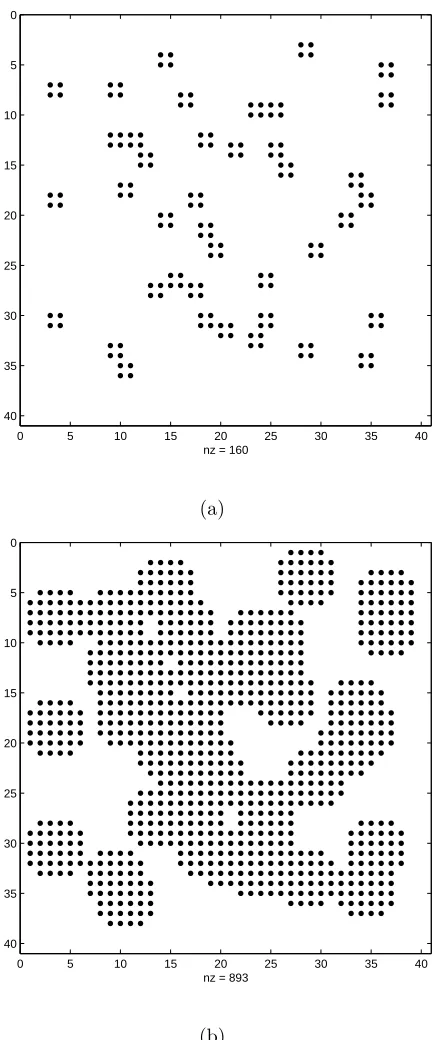
2.2 Partial configuration generated in simulations with fiber density being
0.1. (a) A randomly generated fiber configuration with fiber radius 1.
(b) Same configuration as in (a) but with buffer for a radius 2 walker. 9
2.3 Markov Chain model used in simulations. There are 9 different states
in this model. For example, state 5 represents the state in whichxand
y coordinates remain unchanged; state 3 represents the state in which
bothx and y coordinates increase by 1. . . 10
2.4 Example steps for the Markov Chain model. Dark locations are
inac-cessible due to fibers and buffer zones. Arrows show the intended (in
(a)) or actual moving (in (d)-(i)) direction of a walker. (a) A walker is
waiting in state 5 for transition. For both (b) and (c), the walker will
stay at state 5. (d) The walker will go to state 2. (e) The walker will
go to state 6. For (f), (g), (h) and (i), the walker will go to state 3. . 12
2.5 Sample output of linear regression in x, y and z directions. The 3
figures are generated in a single simulation using parameters β=0.15,
λf=2 and λt=1. The curve lines are the squared diffusion distance
d2i(n)(i =x, y, z) and the straight lines are the fitted regression lines.
The regression coefficient b0s are shown. The dash-dot line in (c) is
the theoretical line whereb = 1. The difference between the sampled b
value and the theoretical value 1 is due to the finite grids we used and
finite samples. . . 14
3.1 γplots. (a)γ plotted against differentβ,λf andλt. E.g., “10-1” means
that λf=10 and λt=1. For β= 0 there is only one point which means
that the theoretical ratio of an isotropic diffusion would be exactly 1.
Also, the ratio of “1-3” is included here for verification only. Note that
the replication for each point is 230 except for “1-3” and “10-1”, which
are 10 and 460 respectively. (b) γ plotted against different θ = λf
λt. E.g., ”10” means thatλf=10 and λt=1; ”5” means that λf=10 and λt
=2 or λf=5 and λt =1. The standard deviation for each point is also
shown. . . 18
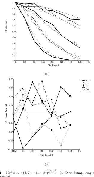
3.2 Model 1. γ(β, θ) = (1−β3)eaβ3θ/2. (a) Data fitting using model 1. (b)
Regression residual. . . 20
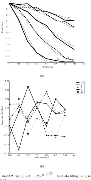
3.3 Model 2. γ(β, θ) = (1−βa)e(1−e(6βbθ ))
. (a) Data fitting using model 2.
(b) Regression residual. . . 21
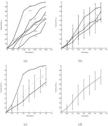
3.4 The estimates of pt. (a) The estimate of pt against 9 combinations of
λf and λt. (b) The estimate of pt averaged across same λf. (c) The
estimate ofptaveraged across sameλt. (d) The estimate ofptaveraged
across combinations of λf and λt against β. . . 23
List of Tables
1.1 Diameters of collagen fibrils in articular cartilage and dextrans used in
FRAP studies. . . 4
Chapter 1
Introduction: Anisotropic Diffusion in FRAP
FRAP (Fluorescence Recovery After Photobleaching) techniques can be used to
measure the effective diffusion coefficients of tracer molecules within biological
mate-rials like articular cartilage [1]. Because of the existence of collagen fibers, molecules’
diffusion will be anisotropic, which means that the effective diffusion coefficients for
the principal directions of the diffusion tensor may be different. It is known that
collagen density and tissue permeability can be determined from diffusion of tracer
molecules which may be measured by using FRAP [1]. Experimentalists are now
in-terested in uncovering the relationships between the anisotropic diffusion of molecules
and the structural anisotropy of cartilage matrix. Can we feasibly use the same
tech-nique to measure collagen anisotropy? Here collagen anisotropy means the axial
differences of collagen’s 3-dimensional space distribution.
From the continuum perspective, the characteristic equation for the diffusion
pro-cess without drift can be written as: [2, 3]
∂C
∂t + (
∂Fx
∂x +
∂Fy
∂y +
∂Fz
∂z ) = 0, (1.1)
where C is the time dependent concentration (or distribution) of the diffusing
2
the assumptions for the fluxes are:
−Fx =Dxx∂C∂x +Dxy∂C∂y +Dxz∂C∂z
−Fy =Dyx∂C∂x +Dyy∂C∂y +Dyz∂C∂z
−Fz =Dzx∂C∂x +Dzy∂C∂y +Dzz∂C∂z,
(1.2)
where Dij(i, j = x, y, z) is the diffusion coefficient of the flux function Fi for axis j.
If we assume axial independence and that the principal diffusion directions are the
same as the coordinate axes, we can write the coefficient matrix D as
Dx 0 0
0 Dy 0
0 0 Dz
(1.3)
Then by plugging the flux functions (1.2) into the characteristic equation (1.1), we
can get
∂C
∂t =
∂ ∂x(Dx
∂C ∂x) +
∂ ∂y(Dy
∂C ∂y) +
∂ ∂z(Dz
∂C
∂z), (1.4)
where Di(i=x, y, z) is the diffusion coefficient for the specific axis i. In our
simula-tions, we assume that the Dis are spatially uniform (not always true), which means
that
∂C
∂t =Dx
∂2C
∂x2 +Dy
∂2C
∂y2 +Dz
∂2C
∂z2. (1.5)
With the particles being dispersed from the origin, the normalized solution to (1.5)
using vector-tensor form is [6]
C(x0, t) =
1
(2πt)3/2det(2D)1/2e
−21tx0T(2D)−1x0
3
where x0 = (x, y, z) is the space coordinate. The level surfaces of this solution are
ellipsoids, not spheres, unless the diffusion is isotropic. Experimentally, if we observe
elliptical shapes for level surface projections in FRAP, we know that there exist
differences among the D’s. But the diffusion equation cannot give us the information
of the relationships between the D’s and the cartilage matrix. Here we are more
interested to investigate the relationship between the D’s anisotropy and the degree
of fiber anisotropy using discretized simulation approach. We hypothesize that the
relationship between fiber anisotropy and diffusion anisotropy depends non-trivially
on two factors only:
1. Fiber volume fraction (referred to as fiber density, denoted by β).
2. Diameter ratio of fiber and tracer molecules (diameter of fibers is denoted by
λf, diameter of tracer molecules is denoted byλt, and diameter ratio is denoted
by θ = λf
λt).
In this study, we will examine the relationship between anisotropy of collagen fibers
and anisotropy of the tracer molecule diffusion coefficients. For simplicity, we look
at the extreme case of complete alignment of infinitely long fibers in the z direction,
which means that we have the same configurations for different z values. Typically,
dextrans are used as diffusive tracer molecules. Tracer molecules are assumed to be
4
radii are assumed to be the same and all tracer radii are the same. See Figure 1.1 for
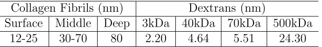
an example of part of a configuration. Table 1.1 gives the actual diameters of collagen
Figure 1.1 Cylinders represent identical collagen fibers which are parallel oriented in
thez direction and randomly distributed in thexy plane.
fibrils at different depth in articular cartilage and the size of dextran molecules used
in experiments [1]. It can be seen that approximately the diameter ratios for collagen
fibrils and dextrans range from 1:2 to 40:1. 9 combinations of fiber and dextran radius
are used in the simulations, including 1:2, 2:4, 1:1, 2:2, 2:1, 4:2, 5:1, 10:2 and 10:1.
Here 1:2 means that fiber radius is h and dextran (walker) radius is 2h, where h is
the grid length. Other combinations are defined in the same way.
Collagen Fibrils (nm) Dextrans (nm)
Surface Middle Deep 3kDa 40kDa 70kDa 500kDa
12-25 30-70 80 2.20 4.64 5.51 24.30
Chapter 2
Methods
The Monte Carlo method was used to simulate the 3-dimensional anisotropic
diffusion of walkers in the fluid between collagen fibers. We discretized the fiber space
using rectangular grids. The grid cell length h=hx =hy =hz is chosen to be 1 and
is used as the reference value for all the data in the simulation. Given fiber density
β, fiber diameterλf, and tracer molecule diameterλt, 230 fiber configurations which
are not totally blocking were generated randomly for each set of 3 parameter values.
For each configuration, a Markov Chain model was used to simulate the random walk
process for 100 walkers within 800 steps. Squared diffusion distance d2i(n)(i=x, y, z)
was used to estimate the corresponding Di using linear regression with respect to
time (step) n for each walker. All walkers’ d2i(n) were averaged to get the pooled
estimates of Di for each configuration. Diffusion coefficient ratios γj = DDjz(j =x, y)
were then calculated to measure fiber anisotropy. Using symmetry we assumed that
Dx =Dy, so we calculated the diffusion ratio as γ = (Dx+DDzy)/2. Different estimates
of γ for all the 230 configurations were then averaged to get the pooled estimates of
γ for same β, λf and λt. After running the simulations for different sets of β, λf
and λt, the relationship between the estimates of γ and the influencing factorsβ, λf
6
Also, because the randomly generated configurations may have trapping regions (i.e.,
extreme cases which restrict the walkers’ diffusion from the very beginning), we only
used the non-trapping configurations in our simulations to avoid axial bias and also
studied the relationship between the probability of generating trapping configurations
and the geometric factors.
2.1
Structure of Domain
Samples of tissue are modeled as cubes with all edges’ length equal 500h.
Practi-cally, this size is big enough to allow walkers moving within 800 steps without running
into the boundary. The origin is set to be in the center of the cube. If there are two
“center” grid points (which is our simulated case), the one with smaller grid index is
used. Walkers’ step length is set to be one grid length h. All walkers start from the
origin. Each walker walks on grid points only. Both fibers and walkers are modeled
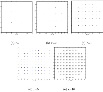
as circles in the xy plane, and are approximated by discretized disks. Examples of
disks with different radius are shown in Figure 2.1. Positions of fibers’ centers are
randomly generated using the uniform random number generator in M AT LABr.
Fibers are not allowed to form intersections with each other. Fibers are not allowed
to intersect the boundaries. A configuration generated will have 0 or 1 for all the
grid points. Here 0 means that a grid point is available for walker’s moving in; 1
means that a grid point is occupied by the fibers already. Also, notice that walkers
7
0 0.5 1 1.5 2 2.5 3
0 0.5 1 1.5 2 2.5 3
nz = 4
(a) r=1
0 0.5 1 1.5 2 2.5 3 3.5 4 4.5 5
0 0.5 1 1.5 2 2.5 3 3.5 4 4.5 5
nz = 12
(b) r=2
0 1 2 3 4 5 6 7 8 9
0 1 2 3 4 5 6 7 8 9
nz = 52
(c) r=4
0 1 2 3 4 5 6 7 8 9 10 11
0 1 2 3 4 5 6 7 8 9 10 11
nz = 80
(d) r=5
0 2 4 6 8 10 12 14 16 18 20
0 2 4 6 8 10 12 14 16 18 20
nz = 316
(e) r=10
8
center of the walker may not penetrate. We also designate the grid points within the
boundary layer with 1, then we can track the movement of an equivalent walker with
zero radius. The boundary layers of different fibers may overlap with each other. The
boundary layers are not allowed to intersect the boundaries either. An example of
the randomly generated configurations is shown in Figure 2.2. Because the randomly
generated configurations may have trapping zones, which we define as extreme cases
when the walker’s diffusion is obstructed around the origin, we only use the
non-trapping configurations in our simulations to avoid bias of obstruction for either xor
y direction.
2.2
Structure of Random Walk
The effects of collagen obstructing dextran diffusion in the xy plane can be
illus-trated by comparison with free diffusion in thezdirection. Diffusion in thez direction
is modeled as a simple random walk because there are no obstructions along thezaxis.
Simple random walk here means thatP r(Zn+1 =Zn+ 1) =P r(Zn+1=Zn−1) = 12.
A more complicated Markov Chain model is used to simulate the diffusion process
in the xy plane, see Figure 2.3. For this Markov Chain model, there are 9 different
states. We can number the states from 1 to 9. Every two different states are
inter-connected with self loop allowed, which means that a walker can go from its current
9
0 5 10 15 20 25 30 35 40
0
5
10
15
20
25
30
35
40
nz = 160
(a)
0 5 10 15 20 25 30 35 40
0
5
10
15
20
25
30
35
40
nz = 893
(b)
10
Figure 2.3 Markov Chain model used in simulations. There are 9 different states in
this model. For example, state 5 represents the state in which x and y coordinates remain
unchanged; state 3 represents the state in which both xand y coordinates increase by 1.
1. First, generate 3 independent uniform random numbers. Using them to
deter-mine the direction of movement forx, y and z axes separately. Let us consider
the xy plane first. For example, suppose state 5 is the resting state waiting for
transition, and the direction is targeted towards state 2 and state 6 now. See
Figure 2.4(a).
2. If site 2, 3, 6 are all obstructed, or only site 3 is obstructed, stay at state 5. See
Figure 2.4(b-c).
3. If only site 2 is not obstructed, go to state 2. See Figure 2.4(d).
4. If only site 6 is not obstructed, go to state 6. See Figure 2.4(e).
5. Otherwise, go to state 3. Note that there are 4 different kinds of conditions
11
6. Along the z axis, there are no obstructions, so the walker always moves up or
down and never stay still.
In thez direction, walkers can either go up or down; in thexandydirection, walkers
can either go forward, backward, or stay still.
2.3
Structure of Simulations
The simulations randomly generate 230 non-trapping fiber configurations for each
of 7 selected fiber densities (0.05, 0.10, · · · ,0.35) and 9 combinations of fiber and
dextran radius (2:4, 1:2, 2:2, 1:1, 4:2, 2:1, 10:2, 5:1 and 10:1). Note that fiber density
βis defined as area fraction, which after discretization is point fraction. For one single
configuration, total simulation step n is 800 and 100 replications (walkers) are used.
Note that if we consider the radius ratio of fiber to walker, we have 5 different ratios:
0.5, 1, 2, 5 and 10. In order to make the data balanced for the ratios, we actually
run 2*230=460 non-trapping fiber configurations for the 10:1 case.
2.4
Probability Models and Statistical Methods
A walker’s movement in the z direction can be modeled as a simple random walk.
The position of the walker after thenth step differs from its position after the (n−1)th
step by ±h:
z(n) =z(n−1) +δn, (2.1)
where P r(δn=h) =P r(δn=−h) = 12, n ≥1, z(0) = 0. So
12
(a) (b) (c)
(d) (e) (f)
(g) (h) (i)
13
The expectation of z(n)2 is
E(z(n)2) =E(z(n−1)2) +E(2z(n−1)δn) +E(δn2) =E(z(n−1)2) +h2 (2.3)
By induction, we know that [4]
E(z(n)2) =h2n = 2Dzn=bn (2.4)
where Dz = h
2
2 =
1
2(note that h = 1) and b is the regression coefficient. We know
that Dz is in fact the diffusion coefficient in equation (1.5) [4]. The squared diffusion
distance d2z(n) can be used to estimate E(z(n)2):
d2z(n) =bn+Yn, (2.5)
where Yn = 4h2(Xn − n2)2 −h2n and Xn =
n P i=1
(δi+h)
2h ∼ binomial(n,
1
2). Although
Yn is not to be independent normal error, we can still use ordinary linear regression
on d2z(n) with step n to estimate Dz. Note that the estimated diffusion coefficient
Dz is only half of the linear regression coefficient b. In both x and y directions,we
assume that the diffusion also follows equation (2.4), while values of Dx and Dy are
now dependent on β,λf and λt.
In our model, we assume that Dx and Dy have no significant difference averaged
over all possible configurations, which means that in the xy plane, the diffusion is
isotropic. Although there exist some configurations for which the estimates ofDx and
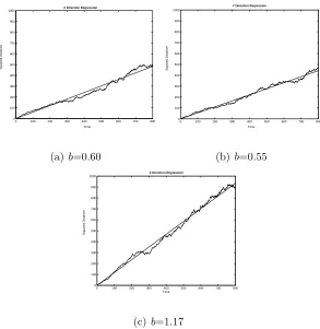
Dy are quite different, these estimates are still kept because we are only interested in
the magnitude of Dx and Dy compared with Dz. See Figure 2.5 for an example of
14
0 100 200 300 400 500 600 700 800
0 100 200 300 400 500 600 700 800 900 1000
X Direction Regression
Time
Squared Distance
(a) b=0.60
0 100 200 300 400 500 600 700 800
0 100 200 300 400 500 600 700 800 900 1000
Y Direction Regression
Time
Squared Distance
(b)b=0.55
0 100 200 300 400 500 600 700 800
0 100 200 300 400 500 600 700 800 900 1000
Z Direction Regression
Time
Squared Distance
(c) b=1.17
Figure 2.5 Sample output of linear regression in x,y and z directions. The 3 figures
are generated in a single simulation using parameters β=0.15, λf=2 and λt=1. The curve
lines are the squared diffusion distanced2i(n)(i=x, y, z) and the straight lines are the fitted
regression lines. The regression coefficient b0s are shown. The dash-dot line in (c) is the
theoretical line whereb= 1. The difference between the sampledbvalue and the theoretical
15
above output, the estimates ofDx andDy may be quite different for a single
configu-ration. It happens mainly because of randomly generated configuration bias in either
x or y direction. We assume that by averaging the estimates of different randomly
generated configurations, this kind of bias can be balanced without influencing the
relationship of diffusion coefficients and the factors β, λf and λt. Dx and Dy are
averaged to estimate the diffusion coefficient ratioγ using γ = (Dx+Dy)/2
Dz .
2.5
Trapping Probability
p
t’s Estimation
Because the configurations are randomly generated, there could be configurations
which have no spanning path to allow walkers to diffuse away starting from the
origin, especially for high density of fibers. Percolation theory can be used to study
when a fiber configuration is macroscopically open to the diffusion phenomenon [5].
Intuitively, there exists a critical value βc for fiber density: when fiber density β >
βc, the configurations are macroscopically closed to diffusion; when β < βc, the
configurations are macroscopically open to diffusion. βc is well below the maximal
packing density, which can be calculated as π
6 ≈ 0.52. Here we are not interested
in finding the critical value βc, because cartilage fiber density falls below 35% of
collagen presumably to stay away from the percolation limit and allow some large
molecules to be able to diffuse. However, we still need to consider the microscopic
trapping phenomenon. This kind of trapping can make the computation of diffusion
16
here to label a configuration as trapping: if after 80 steps (10% of the total steps)
of walking, the standard deviation of the walker’s diffusion coefficients for either x
or y direction is below 0.01h, then the specific configuration is said to be trapping.
Configurations will be continually generated until 230 non-trapping ones are available
for diffusion simulations. We define pt as the probability that a randomly generated
configuration is a trapping one, n as the total configurations generated in order to
Chapter 3
Results
3.1
Diffusion Ratio
γ
’s Dependence on Fiber Density
β
, Fiber
Size
λ
fand Walker Size
λ
tWe define the diffusion coefficient ratio γ as (Dx+Dy)/2
Dz . We also denote fiber density with β, diameter of fibers with λf, and diameter of walkers with λt. In this
study, we want to find the relationship between γ and the influencing factors using
the simulated data. See Figure 3.1(a) for γ plotted against different combinations of
β,λf and λt averaged across 230 different configurations. From Figure 3.1(a), we see
that it is acceptable that the curves with same fiber-walker radius ratio θ = λf
λt can be grouped together. See Figure 3.1(b) for γ plotted against different fiber/walker
size ratio θ averaged across 460 different configurations. We can see thatγ decreases
as β increases and θ decreases. Also, it shows that for θ =5 and 10, γ curves have
relatively bigger estimation error; while forθ = 0.5, γ curve is estimated pretty well.
Two curve fitting models are shown below for the data in Figure 3.1(b).
Model 1: it is intuitively attractive to fit the data in Figure 3.1(b) using an
exponential decaying function [7] likeγ(β, θ) = (1−β3)eaβ 3/2
θ , whereais the parameter
to be fitted. Note that we require a < 0 since for a given β, as θ increases, γ
increases. Also the function satisfies the boundary conditions, namely γ(1, θ) = 0
18
0 0.05 0.1 0.15 0.2 0.25 0.3 0.35 0.4
0 0.1 0.2 0.3 0.4 0.5 0.6 0.7 0.8 0.9 1
Fiber Density β
Diffusion Ratio γ 10−1 5−1 10−2 4−2 2−1 1−1 2−2 1−2 2−4 1−3 (a)
0 0.05 0.1 0.15 0.2 0.25 0.3 0.35 0.4
0 0.1 0.2 0.3 0.4 0.5 0.6 0.7 0.8 0.9 1
Fiber Density β
Diffusion Ratio γ 10 5 2 1 0.5 (b)
Figure 3.1 γ plots. (a) γ plotted against different β, λf and λt. E.g., “10-1” means
that λf=10 and λt=1. Forβ = 0 there is only one point which means that the theoretical
ratio of an isotropic diffusion would be exactly 1. Also, the ratio of “1-3” is included here for verification only. Note that the replication for each point is 230 except for “1-3” and
“10-1”, which are 10 and 460 respectively. (b) γ plotted against different θ = λf
λt. E.g.,
”10” means that λf=10 and λt=1; ”5” means that λf=10 and λt =2 or λf=5 and λt =1.
19
The fittedais −13.3±0.4 andR2 = 0.89. If we use unweighted regression, the fitted
a is −13.1±0.4 and R2 = 0.99. Only weighted regression results are presented here.
See Figure 3.2 for the data with fitted curves residuals. No trends seem to exist for
the residuals. Also, the residuals’ magnitude is less than 0.08.
Model 2: we can also fit a two-parameter model using γ(β, θ) = (1−βa)e(1−e(6βbθ )),
wherea, bare the parameters to be fitted. Note that the model automatically suffices
that given β, as θ increases, γ increases. Also the function satisfies the boundary
conditions, namelyγ(1, θ) = 0 andγ(0, θ) = 1. The inverse of γ’s standard deviation
is still used as regression weight. The fitted a is 1.7±0.1, the fitted b is 1.30±0.02
andR2 = 0.92. If we use unweighted regression, the fittedais 1.7±0.1, the fittedbis
1.29±0.01 and R2 = 0.99. Only weighted regression results are presented here. See
Figure 3.3 for the data with fitted curves and residuals. No trends seem to exist for
the residuals. Also, the residuals’ magnitude is less than 0.08. It is also interesting
that weighted and unweighted regression give almost the same fits.
It is clear that model 2 works better than model 1. We can see that the fittings
work much better at high level of density because we have used the inverse of γ0s
standard deviation as the regression weight and the standard deviation is smaller at
high β. Experimentally, we are most interested in the cases where fiber density is
around 20% and the diffusion ratio is relatively small. Both models presented are
20
0 0.05 0.1 0.15 0.2 0.25 0.3 0.35 0.4
0 0.1 0.2 0.3 0.4 0.5 0.6 0.7 0.8 0.9 1
Fiber Density β
Diffusion Ratio γ 10 5 2 1 0.5 (a)
0.05 0.1 0.15 0.2 0.25 0.3 0.35 0.4 −0.08 −0.06 −0.04 −0.02 0 0.02 0.04 0.06 0.08
Fiber Density β
Regression Residual 0.5 1 2 5 10 (b)
Figure 3.2 Model 1. γ(β, θ) = (1−β3)eaβ
3/2
θ . (a) Data fitting using model 1. (b)
21
0 0.05 0.1 0.15 0.2 0.25 0.3 0.35 0.4
0 0.1 0.2 0.3 0.4 0.5 0.6 0.7 0.8 0.9 1
Fiber Density β
Diffusion Ratio γ 10 5 2 1 0.5 (a)
0.05 0.1 0.15 0.2 0.25 0.3 0.35 0.4 −0.08 −0.06 −0.04 −0.02 0 0.02 0.04 0.06 0.08
Fiber Density β
Regression Residual 0.5 1 2 5 10 (b)
22
3.2
The Estimate of Trapping Probability
p
t’s Dependence
on Fiber Density
β
, Fiber Size
λ
fand Walker Size
λ
tFor the trapping probability pt, let n be the number of total configurations
generated in order to get m non-trapping ones. We know that n has a negative
binomial(m,1−pt) distribution. We may conclude that the frequency estimate of pt
is n−m
n , which is also the MLE of pt .
See Figure 3.4 for the estimate of pt(β) averaged across different combinations of
λf and λt. From the figure, we can see that pt is non-decreasing withβ as expected,
and the averaged estimation curve has a sigmoid shape. Given a fiber density β,ptis
almost non-increasing forλf, which means that fibers with bigger sizes make diffusion
easier. Also, given a fiber density β, pt is non-decreasing for λt, which means that
tracer molecules with smaller sizes make diffusion easier. Approximately, βc is about
0.50 for our model when the trapping probabilitypt is almost 1 for all combinations.
3.3
Discussion
It is quite clear that the diffusion ratio γ decreases as fiber density β increases.
Also, for a specific fiber density, the curves increase as θ increases. This means
that the relatively larger tracer molecules are preferred for detecting fiber anisotropy,
which is consistent with the results of hindered diffusion in porous materials [8]. As
we have seen, our regression models give satisfactory outcomes for fitting the
23
0 0.05 0.1 0.15 0.2 0.25 0.3 0.35 0.4 0 0.1 0.2 0.3 0.4 0.5 0.6 0.7 0.8 0.9 1
Fiber Density β
Trapping Ratio p
t 2−4 1−2 2−2 2−1 4−2 10−2 5−1 10−1 1−1 (a)
0 0.05 0.1 0.15 0.2 0.25 0.3 0.35 0.4 0 0.1 0.2 0.3 0.4 0.5 0.6 0.7 0.8 0.9 1
Fiber Density β
Trapping Ratio p
t 2 1 4 5 10 (b)
0 0.05 0.1 0.15 0.2 0.25 0.3 0.35 0.4
0 0.1 0.2 0.3 0.4 0.5 0.6 0.7 0.8 0.9 1
Fiber Density β
Trapping Ratio p
t
4
2
1
(c)
0 0.05 0.1 0.15 0.2 0.25 0.3 0.35 0.4 0 0.1 0.2 0.3 0.4 0.5 0.6 0.7 0.8 0.9 1
Fiber Density β
Trapping Ratio p
t
(d)
Figure 3.4 The estimates of pt. (a) The estimate of pt against 9 combinations of λf
and λt. (b) The estimate of pt averaged across same λf. (c) The estimate of pt averaged
across same λt. (d) The estimate of pt averaged across combinations of λf and λt against
24
would prefer model 1 to be used instead because of parsimony and simplicity factors.
Numerically, both models are good enough to be used for pre-experiment prediction
and post-experiment validation. The simulated relationship between γ and β, θ can
be used to give approximated size information for choosing different dextrans. For
instance, if the cartilage is 20% collagen and the experimenters want to be able to
detect anisotropy withγ = 0.3, they should make sure to use a dextran of at least the
diameter of the fibers. If they need aγ of 0.1, they would need to use a dextran twice
as big as the fiber diameter at 20% collagen density. We can also use the simulated
results to validate (or invalidate) the experimental outcomes.
The simulations used here neglect molecule-molecule interactions, so the results
may be accurate only for tracer molecules of low density [8]. Also, in articular
car-tilage, other biological molecules may also influence the diffusion of tracer molecules
25
References
1. Leddy, H.A. and F. Guilak, ”Diffusion Coefficients Vary with Depth in Articular Cartilage”, Annals of Biomedical Engineering 29(S1): S30, 2001.
2. J.Crank, The Mathematics of Diffusion. Clarendon Press, Oxford: 1956.
3. H.S.Carslaw., J.C.Jaeger, Conduction of Heat in Solids. Clarendon Press, Ox-ford: 1959.
4. Howard C. Berg,Random Walks in Biology. Princeton University Press, Prince-ton, N.J.: 1983.
5. Muhammad Sahimi,Applications of Percolation Theory. Taylor & Francis, Lon-don; Bristol, PA : 1994.
6. Anders Stockmarr, ”The Distribution of Particles in the Plane Dispersed by a Simple 3-dimensional Diffusion Process”, J.Math.Biol. 45, 461-469, 2002.
7. Samiul Amin, ”Brownian Motion in Viscoelastic Media”, Thesis (Ph.D.), North Carolina State University, 2002.