Blood pressure and blood flow variation during postural change from sitting to standing: model development and validation

Blood Pressure and Blood Flow Variation during

Postural Change from Sitting to Standing: Model

Development and Validation

Department of Mathematics &

Center for Resarch in Scientific Computation North Carolina State University

Raleigh, NC 27695 email: msolufse@math.ncsu.edu

Phone: (919) 515 2678, Fax: (919) 513 7336 Johnny T. Ottesen

Department of Mathematics and Physics Roskilde University, Roskilde, Denmark Hien T. Tran and Laura M. Ellwein

Department of Mathematics &

Center for Resarch in Scientific Computation North Carolina State University, Raleigh, NC 27695

Lewis A. Lipsitz

Hebrew SeniorLife, Research and Training Institute, Division of Gerontology, Beth Israel Deaconess Medical Center,

and Harvard Medical School, Boston, MA 02215 Vera Novak

Division of Gerontology Beth Beth Israel Deaconess Medical Center and Harvard Medical School, Boston, MA 02215

Abstract— Short term cardiovascular responses to

pos-tural change from sitting to standing involve complex interactions between the autonomic nervous system that regulates blood pressure, and cerebral autoregulation that maintains cerebral perfusion. We present a mathematical model that can predict dynamic changes observed in beat-to-beat arterial blood pressure and middle cerebral artery blood flow velocity during postural change from sitting to standing. Our cardiovascular model utilizes 11 compartments to describe blood pressure, blood flow, compliance and resistance in the heart and systemic circulation. To include dynamics due to the pulsatile nature of blood pressure and blood flow, resistances in the large systemic arteries are modeled using nonlinear functions of pressure. A physiologically based sub-model is used to describe effects of gravity on venous blood pooling during postural change. Two types of control mechanisms are included: (i) Autonomic regulation mediated by sym-pathetic and parasymsym-pathetic responses that affect heart rate, cardiac contractility, resistance, and compliance. (ii) Autoregulation mediated by responses to local changes in myogenic tone, metabolic demand, and concentration

of carbon dioxide (CO2) that affect cerebrovascular

re-sistance. Finally, we formulate an inverse least squares problem for parameter estimation and to demonstrate that our mathematical model is in agreement with physiological data obtained from a young subject during postural change from sitting to standing.

I. INTRODUCTION

Orthostatic intolerance disorders, which are common in every age, are difficult to diagnose and treat. Typi-cally, these disorders whose clinical manifestations in-clude dizziness, syncope, orthostatic hypotension, falls, and cognitive decline are a result of several biological mechanisms. To develop better strategies to treat and diagnose orthostatic intolerance, it is important to un-derstand the underlying mechanisms leading to these disorders. One of the main mechanisms involved is the short term cardiovascular regulation of blood flow to the brain, which include both autonomic regulation and cerebral autoregulation. The overall goal of this work is to develop a mathematical model that can predict dynamics in observed cerebral blood flow and peripheral blood pressure data, and to propose mechanisms that can explain the interaction between autonomic regulation and cerebral autoregulation. To this end we have developed a mathematical model that can predict these two regulatory mechanisms. To validate the model we compare model predictions with arterial finger blood pressure paf, and middle cerebral artery blood flow velocityvacp measure-ments from a young subject.

Upon standing from a chair, blood is pooled in the lower extremities due to gravitational forces. As a result, venous return is reduced, which lead to a decrease in cardiac stroke volume, a decline in arterial blood pressure, and an immediate decrease of blood flow to the brain. The reduction in arterial blood pressure un-loads the baroreceptors located in the carotid and aortic walls, which leads to parasympathetic withdrawal and sympathetic activation through baroreflex-mediated au-tonomic regulation. Parasympathetic withdrawal induces fast (within 1-2 cardiac cycles) increases in heart rate, while sympathetic activation yields a slower (within 6-8 cardiac cycles) increase in vascular resistance, vascular tone, cardiac contractility, and a further increase in heart rate [4], [7], [37]. Simultaneously, cerebral autoregula-tion, mediated by changes in CO2, myogenic tone, and

metabolic demand leads to vasodilation of the cerebral arterioles [2], [18], [34], [38].

Our mathematical model includes two sub-models: (i) a cardiovascular model that can predict blood pressure and blood flow velocity during sitting (for t≤60 sec.), and (ii) a control model that can predict autonomic and cerebral regulatory mechanisms during postural change from sitting to standing. Both sub-models are based on the same closed-loop compartmental model with 11 compartments that represent the heart and systemic circulation. Our previous work [27], [29] also used compartmental models to describe the dynamics of the

cardiovascular system. The model in [27] used an open-loop model (the 3-element windkessel model) to analyze dynamics of cardiovascular control. This model used arterial blood pressure measured in the finger as an input to predict model parameters that describe dynamics of cerebral vascular regulation for young people. These parameters were obtained by minimizing the error be-tween computed and measured middle cerebral arterial blood flow velocity. Consequently, no equations were used to describe possible mechanisms of the underlying regulation. To further advance this study, we recently developed a 7 compartmental closed-loop model, that can predict the dynamics observed in the data. This model did not rely on an external input, but included a model that describe the pumping of the left ventricle. In addition, the 7 compartmental model included simple equations that describe the short term regulation. This model was able to accurately predict dynamics of both cerebral blood flow velocity and arterial blood pressure during sitting (fort <60 sec.) and standing (for t >80 sec), as well as the mean values during the transition (for 60< t <80sec.), but it was not able to predict detailed dynamics during the transition region. Furthermore, we were not able to obtain adequate filling of the left ventri-cle. To obtain a more accurate model we developed the 11 compartmental model described in this work, which overcome limitations of the 7 compartmental model as described below.

To obtain adequate filling of the left ventricle we added a compartment that represents the left atrium. In the 7 compartmental model we used the blood pressure in the upper body to validate the model against data, which are measured in the finger. The pulse pressure (systolic minus diastolic pressure) in the upper body is too wide and very sensitive to parameter changes. Hence, to improve our model we included a compartment that represents the arteries in the finger. In addition, we added two small compartments that represent the aorta and vena cava. These compartments were primarily added to improve model simulation stability. In summary, the improvements discussed above have led to the addition of 4 additional compartments. Furthermore, the 7 compart-mental model was not able to predict pulse pressure reg-ulation immediately following standing. To compensate for this we have modeled resistance of the large arteries using nonlinear functions of pressure. Finally, to obtain accurate widening of the blood flow velocity, a feature that our 7 compartmental model was not able to predict, we devised an empirical model of autoregulation, and a physiological model that can predict pooling of blood in lower extremities, due to effects of gravity.

control modeling, e.g., [10], [11], [12], [30], [44] is based on predictions of mean values for arterial blood pressure and cerebral blood flow velocity. Consequently, these models can not predict the pulsatile dynamics of the cardiovascular system. These models use opti-mal control to minimize the deviation between some observed quantity (e.g., arterial blood pressure) and a given set-point. While this strategy can provide good parameter estimates, optimal control models do not de-scribe the underlying physiological mechanisms. Other modeling strategies have been proposed in the work by Melchior [19], [20] and Heldt [8], who devise pulsatile models that include pulsatility, autonomic regulation, and effects of gravity. The latter was done by changing the reference pressure outside the compartments. However, these models do not include effects of autoregulation. One way to model the effect of autoregulation is to let the cerebrovascular resistance be a function of time as suggested by Ursino [39]. However, this work does not include the effects of autonomic regulation.

A second group of models has described parts of the control system without validation against experi-mental data, e.g., [5], [19], [20], [21], [31], [32], [35], [40], [41], [42], [43]. These models used a closed-loop compartmental description of the cardiovascular system combined with physiological descriptions of the control. While these models can provide qualitative analysis of the system they cannot be used for quantitative compar-isons with data. Furthermore, most of the models in the second group describe the effects of autonomic regula-tion without including the effects of cerebral autoregu-lation. In contrast, our model includes both autonomic and cerebrovascular regulations and provides quantitative comparisons with physiological data.

II. MODELINGBLOODPRESSURE AND BLOODFLOW

VELOCITY

A. A Compartmental Model for the Cardiovascular Sys-tem

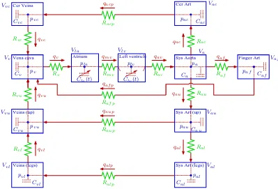
Our cardiovascular model is based on a closed-loop model with 11 compartments. This model is designed to predict blood pressure and volumetric blood in the left atrium, the left ventricle, aorta, vena cava, arteries and veins in the upper body, the lower body, and the head, as well as arteries in the finger, see Fig. 1. Each compartment represents all vessels in areas of similar pressure. Hence, in its simplest form the systemic circuit could consist of one arterial compartment (high pressure) and one venous compartment (low pressure). In our model, we include 5 arterial compartments and 4 venous compartments.

The 11 compartments depicted in Fig. 1 are chosen to ensure that the level of detail in the model is adequate to describe the complex dynamics observed in the data and at the same time not too complex to be solved computationally. Four compartments that represent the upper body and the legs are included to model venous pooling of blood and sympathetic contraction of the vascular bed. Two compartments that represent the brain are included to model effects of cerebral autoregulation and to enable model validation against cerebral arterial blood flow velocity measurements. One compartment that represents the finger is included to enable model validation against arterial blood pressure measured in the finger. To determine cardiac output and venous return, two compartments are included to represent the aorta and vena cava. Finally, to obtain a closed-loop model it is necessary to include a source (the heart) that pumps blood through the system. Consequently, two compart-ments are included to represent the left atrium and the left ventricle. Our previous work [29] only included the left ventricle, but without an atrium it is not possible to obtain adequate filling of the heart.

The major system not included in our model is the pulmonary circulation. Addition of compartments that represent the pulmonary circulation would require more parameters, which would increase the computational complexity. Instead, the pulmonary circulation is rep-resented as a resistance between vena cava and the left atrium.

To study dynamics of postural change from sitting to standing it is not important to know how blood is distributed among various inner organs. Hence, the upper body is simply represented by an arterial and a venous compartment. Each compartment is represented by a compliance element (inverse elasticity) and is separated by resistance to flow. The design of the systemic cir-culation with arteries and veins separated by capillaries provides some resistance and inertia to the volumetric flow rate. In our model we include effects of resistance between compartments but neglect effects due to inertia. The major resistance to flow is located in peripheral regions between compartments that represent arteries and veins. Compartments that represent large conduit vessels are also separated by resistances that represent the overall resistance of the compartment. Resistances between conduit vessels are very small compared with the peripheral resistances.

The description of blood pressure and volumetric flow rate in a system comprised of compliant compartments (capacitors) and resistors are equivalent to that of an electrical circuit, see Fig. 1, where blood pressure p

Finger Art

Veins (legs)

Vena cava Atrium

Sys Art (legs) Sys Art (up) Cer Art

Sys Aorta Cer Veins

Veins (up)

Left ventricle

qal qaf p

Raup

Racp qacp

Rac

Rav qav

Caf

Vaf

Raf qaf

qau Rau

Cau

pv

Vvl

Cvl

pvu

pvc

Vv

pvl

Cal

pac

Val

Vau

pal

pla plv pa

Clv(t)

qac

qalp qaup

Vac

Cvc

Cv

Vvc

Vla

Cla(t)

Cvu

Vvu

Cac

Ca

Va

paf

pau

Ralp

Ral

Rvc qvc

qvu

Rvu

qvl

Rvl

Rmv

Rv

qmv qv

Vlv

Raf p

Fig. 1. Compartmental model of the systemic circulation. The model contains 11 compartments. 5 compartments represent systemic arteries (the brain, upper body, lower body, aorta and the finger), 4 compartments represent the systemic veins (the brain, upper body, lower body, and vena cava), and 2 compartments represent the left atrium and left ventricle. Since the pulmonary system is not included, the systemic veins are directly attached to the left ventricle. Each compartment includes a capacitor to represent the compliant volume of the arteries or veins. All compartments are separated by resistors representing resistance of the vessels. Furthermore, the compartment representing the left ventricle has two valves (the aortic valve and the mitral valve). Following terminology from electrical circuit theory, the flow between compartments is equivalent to electrical current and the pressure inside each compartment is analogous to voltage. Resistors R [mmHg sec/cm3] are marked with zigzag lines, capacitors C [cm3/mmHg] are marked with dashed parallel lines inside the compartments, while the aortic and mitral valves are marked with short lines inside the compartment that represents the left ventricle. The abbreviations arela left atrium, lv left ventricle,av aortic valve, mvmitral valve, a aorta, auarteries in the upper body, al arteries in the lower body, aup peripheral arteries in the upper body, alpperipheral arteries in the lower body, ac cerebral arteries (in the brain), acpperipheral cerebral arteries,af finger arteries,af p peripheral finger arteries,vl veins in the lower body,vuveins in the trunk and upper body, vvena cava, and vccerebral veins.

rate q [cm3/sec] plays the role of current. To compare our model with data we assume that the diameter of the middle cerebral artery remains constant, such that blood flow velocity can be obtained by scaling volu-metric blood flow by a constant factor that represents the area of the vessel. Recent measurements of middle cerebral artery diameter by magnetic resonance imaging (MRI) combined with transcranial Doppler assessment of cerebral blood flow velocity have demonstrated that the middle cerebral artery diameter does not change despite large changes in cerebral blood flow velocity elicited by stimuli such as lower body negative pressure and CO2

changes [36].

To predict blood pressure and blood flow in and between the compartments we base our model on volume conservation laws [41]. Blood pressure and volumetric blood flow can be found by computing the volume and change of volume for each compartment. The equations that represent the arterial and venous compartments are

similar. For each of these compartments the stressed vol-umeV =Cp[cm3] (volume pumped out during one car-diac cycle), whereC[cm3/mmHg] is the compliance and

p[mmHg] is the blood pressure. The cardiac output from the heart is given byCO =HVstroke [cm3/sec], where

H [beats/sec] is the heart rate andVstroke [cm3/beat] is the stroke volume. For each compartment, the net change of volume is given by

dV

dt =qin−qout, q=

pin−pout

R , (1)

where q [cm3/sec] is determined analogously to Kirch-hoff’s current law andRis the resistance to flow. Several compartments have more than one inflow or outflow. For example, the compartment that represent the aorta has 3 outflows (qout = qaf + qau + qac) while the compartment that represent vena cava has 3 inflows (qin=qaf p+qvu+qvc), see Fig. 1.

During diastole the mitral valve is open while the aortic valve is closed allowing blood to enter the left ventricle. Then, isometric contraction begins, increasing the ven-tricular pressure. Once, the venven-tricular pressure exceeds the aortic pressure, the aortic valve opens, propelling the pulse wave through the vascular system. Note, for healthy young people, both valves cannot be open si-multaneously. To incorporate the state of the valves we have modeled the resistances (Rav andRmv, see Fig. 1) as follows

Rv =min

Rv+e−10(pin−pout),5000

,

where v = mv, av. This equation result in a large resistance (and no flow) while the valve is closed and a small resistance (and normal flow) while the valve is open. The minimum value is introduced to avoid numerical problems due to large numbers.

A system of differential equations is obtained by dif-ferentiating the volume equation V =Cp and inserting (1), i.e.,

dV dt =C

dp dt +p

dC

dt =qin−qout. (2)

The circuit in Fig. 1 gives rise to a total of 9 differential equations in dp/dt, one for each of the arterial and venous compartments. For the two compartments that represent the atrium and the ventricle, differential equa-tions are kept as dV /dt. For these two compartments, blood pressure is computed explicitly as a function of volume, see next section. A complete list of equations can be found in the Appendix.

B. Ventricular and Atrial Contraction

Atrial and ventricular contraction leads to an increase in blood pressure from low values observed in the venous system to high values observed in the arterial system. Our model is based on the work by Ottesen [6], [33]. This model predicts atrial (pla) and ventricular (plv) pressure as a function volume and cardiac activation of the form

p=a(V(t)−b)2+ (c(t)V(t)−d)g(t), p=pla, plv. (3) The parameter a [mmHg/cm3] is related to elastance during relaxation and b[cm3] represents volume at zero diastolic pressure, c(t) [mmHg/cm3] represents contrac-tility, and d [mmHg] is related to the volume dependent and volume independent components of the developed pressure. The activation function g(t), which is defined over the length of one cardiac cycle, is described by a

polynomial of degree (n, m): g(t) =f(t)/f(tp) with

f(˜t) =



  

  

pp ˜

tn_(β−˜t)m

nn_mmh β m+n

im+n 0≤t˜≤β

0 β <˜t≤T.

(4)

T [sec] is the duration of the cardiac cycle, ˜t = mod(t, T) [sec],β(H) [sec] denotes the onset of relax-ation,H = 1/T [1/sec] denotes the heart rate,nand m

characterize the contraction and relaxation phases, and

pp is the peak value of the activation. The ability to vary heart rate is included in the isovolumic pressure equation (3) by scaling time and peak values of the activation function f. The time for peak value of the contraction,

tp [sec], is scaled by introducing a sigmoidal function, that depend on the heart rateH, of the form

tp =tm+

θν

Hν_+θν(tM −tm), (5) whereθrepresents the median andνrepresents the steep-ness, and tm [sec] and tM [sec] denote the minimum and maximum values, respectively. The peak ventricular pressurepp[mmHg] is scaled similarly using a sigmoidal function of the form

pp =pm+

Hη

Hη_+φη(pM −pm), (6)

where φ represents the median and η represents the steepness, pm [mmHg] and pM [mmHg] denote the minimum and maximum values, respectively.

Finally, the time for onset of relaxation β is modeled by

β= n+m

n tp(H). (7)

This equation is obtained by recognizing that the time for peak pressure, tp, is related to the parameter β in the isovolumic pressure model (3). Initial values for all parameters were obtained from the work by Ottesen and Danielsen [33]. In this work, parameters were based on canine data. To obtain human values for the young subject studied in this work, we identified parameters during our model validation. Resulting parameters can be found in Table I.

C. Nonlinear Resistances

Rest. Initial Optimized Heart Initial Optimized Comp.

Rav 0.030 0.1149 av 0.0003 0.0009 Rau 0.072 0.1853 bv 5 4.9122 Ral 0.087 0.0043 cv 6.4 6.9100 Raf 0.183 0.5456 dv 1 0.8310 Rac 0.409 0.3177 nv 2 3.6659 Raup 1.565 1.8565 mv 2.2 1.7369 Ralp 6.522 7.5854 νv 9.9 11.0201 Rapf 17.5 17.8953 θv 0.951 0.9213 Racp 6.696 7.0838 ηv 17.5 17.6658 Rmv 0.007 0.0164 φv 1 1.1560 Rv 0.033 0.0368 tm,v 0.186 0.1310 Rvu 0.001 0.000 tM,v 0.280 0.2305 Rvl 0.174 0.1193 pm,v 0.842 1.1074 Rvc 0.957 1.2875 pm,v 1.158 1.2385 Ca 0.084 0.0732 aa 0.002 0.0002 Cau 0.6160 0.7255 ba 5 4.1074 Cal 0.940 0.9881 ca 6.4 6.4325 Caf 0.174 0.2353 da 1 1.1668 Cac 0.159 0.0892 na 1.9 1.9501 Cv 2.931 2.5181 ma 2.2 1.9767 Cvu 15.276 15.4531 νa 9.9 10.8595 Cvl 6.038 6.2778 θa 1 1.9998 Cvc 2.847 2.3007 ηa 17.5 16.5386

φa 1 2.1152

f act 0.1415 0.2079 tm,a 0.186 0.2487 α 1.4287 2.3220 tM,a 0.280 0.3560 pm,a 0.842 1.0065 pM,a 0.990 1.2100

TABLE I

STEADY STATE PARAMETERS BEFORE AND AFTER OPTIMIZATION. RESISTANCES[MMHG SEC/CM3]ARE USED IN EQUATION(1),

COMPLIANCES[CM3/MMHG]IN EQUATION(2),AND HEART PARAMETERS ARE USED IN EQUATION(3).

Our investigation has shown that such dependencies are important to include in regions that represent vessels with large diameters and high blood pressure (in the large arteries), while they are less important in regions of low blood pressure (in the venous system). Further-more, these “passive” changes in diameters are also negligible in regions with small vessels (in the small arteries and arterioles) where autonomic responses are active and dominate the change in vessel diameters. Our previous work [29] did not include nonlinear arterial resistances and as a result we were not able to obtain a sufficiently wide pulse pressure immediately following postural change from sitting to standing.

To model nonlinearities for these resistances, we base our derivation on Poiseuille’s law. For flow in a cylinder with circular cross-sectional area, Poiseuille’s law

pre-dicts the resistance to flow [14] as

R= 8ηl

πr4,

whereR[mmHg sec/cm3] is the resistance,r[cm] is the radius of the vessel, andη[mmHg sec] is the viscosity of blood, andl [cm] is the length of the cylindrical vessel. Assume a constant length of the vessel, then

1

R ∝r

4_∝V2_∝p2_{. (8)}

squared. For real arteries and veins, the resistance will have maximum and minimum values. Hence, we have chosen to model this nonlinear relation using a sig-moidally decreasing function of the form

R= (RM−Rm)

αk 2

pk_+αk 2

+Rm, (9)

where RM [mmHg sec/cm3] and Rm [mmHg sec/cm3] are the maximum and minimum values that the resis-tances can have, p [mmHg] is the blood pressure in the compartment that precede the resistance (in our imple-mentation the actual blood pressure oscillates too much and as a consequence, for numerical stability, we base the prediction ofRon the corresponding mean arterial blood pressure p¯(t) [mmHg]), resulting ressitance can be seen in Figure 2. As shown in Fig. 3 the mean arterial blood pressure oscillates with the same frequency but with a smaller amplitude than pa.k represents the steepness of the sigmoid, and the parameterα2 is calculated to ensure

that R returns the value of the controlled parameter found during steady state. For k = 2, the slope of the sigmoid approximates the relation in (8). However, the relation in (8) is only valid for a steady flow. Blood flow in arteries is unsteady and the flow through a given vessel depends on the state of the vessel. Consequently, as shown in Table II, we should not expect that k = 2.

In our model 3 resistances are computed as functions of pressure: Ral(¯pau), Rac(¯pa), Raf(¯pa). The resistance of the aorta Rau could also be modeled using this method. Initial investigations showed that other mecha-nisms, e.g., autoregulation or autonomic regulation, may also affect Rau. As a consequence, we have used an empirical model to estimate Rau, see Section III-B.

D. Gravitational Effect

Gravitational effects are essential during postural change from sitting to standing. Consider a cylindrical vessel with length ∆z [cm] and time invariant cross-sectional area A [cm2], i.e., dA/dt = 0. Assume that there is no velocity across the vessel and that the blood pressure is only a function position along the vessel. Hence, dv/dr = 0, v [cm/sec] and r [cm] denotes the velocity and radii, respectively, and the volumetric flow rate becomes q = Av [cm3/sec]. Finally, assume that the drag force due to viscous shear is proportional to

q. Thus, the drag force per cross-sectional area unit is proportional to q, i.e., the drag force can be written as

−RAq, where R [mmHg s/cm3] may be interpreted as the resistance. In steady state, the resistance R is given by Poiseuille’s law

R= 8πη∆z

A2 ,

where η represents the fluid viscosity [23].

To derive the mathematical model we proceed by balancing inertial forces with the drag force, the pressure force, and the gravitational force. The inertial force is given by

Mdv

dt =ρA∆z d dt

_q

A

=ρ∆zdq dt,

where ρ= 1.055 [g/cm3] is the density of the fluid and

M [g] is the mass of the fluid contained in a piece of the vessel with length∆z [cm] and cross-sectional area

A [cm2], see Fig. 4. Thus, Newton’s second law that describes balancing of forces gives

ρ∆zdq

dt = (pin−pout)A+M gcos(ψ)−RAq,

where g = 981 [cm/sec2] is the gravitational accelera-tion. From this it follows that

Ldq

dt =pin−pout+ρg∆h−Rq, (10)

where L =ρ∆z/A [1/sec2] is the inertance and ∆h = ∆zcos(ψ) = hin −hout [cm] is the vertical difference of the vessel inlet (athin wherepin is the inlet pressure andpout is the outlet pressure. During steady state (10) reduces to

q = (pin+ρghin)−(pout+ρghout)

R . (11)

When modeling postural change from sitting to standing we substitute (11) for Kirchhoff’s current law. Notice, in the limit g→0, (11) approaches the normal form of Kirchhoff’s current law given in (1). Also note, in the case of energy conservation (R → 0) Bernoulli’s law for steady flow is recovered; as a result pin+ρghin =

pout+ρghout. Thus Kirchhoff’s current law is still valid if we interpret p as the hydrostatic pressurep+ρgh.

To capture the transition from sitting to standing,

h is defined for the lower-body compartments as the exponentially increasing function

h(t) = hM

1 +e−k(t−Tup−δ), (12)

A

45 50 55 60 65 70 75 80 85 90

0 0.1 0.2 0.3 0.4 0.5

time [sec]

Rau [mmHg s/cm

3]

B

45 50 55 60 65 70 75 80 85 90

0 0.5 1 1.5 2 2.5

time [sec]

Rac [mmHg sec/cm

3]

Fig. 2. “Passive” resistances between compartments that represent the large arteries. The top panel showsRau(t)(fitted, using (19) with

26 values, marked with stars on the figure) and the bottom panel showsRac(t)[mmHg sec/cm

2

] (computed using (9)). Both resistances are depicted for45≤t≤90. Both resistances increase as a response to the decreasing pressure and then decrease to a new steady state value. The resistancesRal(t)andRaf(t)[mmHg sec/cm

2

] are modeled similar toRac(t)and show similar trends.

45 50 55 60 65 70 75 80 85 90

55 60 65 70 75 80 85 90 95 100

time [sec]

pam [mmHg]

Fig. 3. The graph shows the mean arterial pressurepa(t) (written as “pam” on the y-axis) [mmHg] for45≤t≤90. The mean arterial

Initial and optimized regulation parameters

Param. Init. Opt. Param. Init. Opt.

¯

pa 92.8 - k(catr) 2.0 4.58 ¯

pau 90.0 - RM(catr) 4×cssvtr 11.99 τCv 10.0 18.57 Rm(catr) cssvtr/4 0.94 τCa 10.0 13.67 k(Ca) 2.0 0.38 τR 5.0 23.03 CM(Ca) 4×Cass 4.3×10−

2

τS 5.0 0.076 Cm(Ca) Cass/4 4.8×10−

4

hH 50.0 46.73 k(Cau) 2.0 17.22 hk 3.0 3.92 CM(Cau) 4×Causs 1.01 δ 0.4 1.26 Cm(Cau) Causs/4 0.42 k(Ral) 5.0 1.48 k(Cal) 2.0 13.90 RM(Ral) 10×Rssal 1.69 CM(Cal) 4×Calss 15.25 Rm(Ral) Ralss/10 1.1×10−

3

Cm(Cal) Calss/4 0.82 k(Rac) 5.0 8.79 k(Cac) 2.0 4.05 RM(Rac) 10×Rssac 2.49 CM(Cac) 4×Cacss 0.23 Rm(Rac) Racss/10 1.3×10−

2

Cm(Cac) Cacss/4 7.0×10−

2

k(Raf) 5.0 3.83 k(Caf) 2.0 81.34 RM(Raf) 10×Rssaf 1.5×10−

1

CM(Caf) 4×Cafss 0.46 Rm(Raf) Rafss/10 2.9×10−

5

Cm(Caf) Cafss/4 1.7×10−

2

k(Raup) 2.0 5.74 k(Cv) 3.0 0.47 RM(Raup) 4×Rssaup 14.58 CM(Cv) 5×Cvss 15.32 Rm(Raup) Rssaup/4 0.13 Cm(Cv) Cvss/5 0.52 k(Ralp) 5.0 10.57 k(Cvu) 3.0 12.90 RM(Ralp) 10×Rssalp 145.19 CM(Cvu) 5×Cvuss 55.86 Rm(Ralp) Ralpss /10 0.41 Cm(Cvu) Cvuss/5 1.93 k(Raf p) 2.0 3.69 k(Cvl) 3.0 47.93 RM(Raf p) 4×Rssaf p 64.81 CM(Cvl) 5×Cvlss 277.94 Rm(Raf p) Rssaf p/4 0.16 Cm(Cvl) Cvlss/5 0.17 k(cvtr) 2.0 4.62 k(Cvc) 3.0 15.71 RM(cvtr) 4×cssvtr 17.27 CM(Cvc) 5×Cvcss 13.89 Rm(cvtr) cssvtr/4 1.04 Cm(Cvc) Cvcss/5 0.19

TABLE II

OPTIMIZED PARAMETERS. CONSTANTSp¯aANDp¯auDENOTE PRESSURE SET-POINTS USED IN CONTROL-EQUATIONS. TIME-CONSTANTS

τiDENOTE THE TIME DELAY INVOLVED WITH THE CONTROLLED VARIABLES,PARAMETERS FOR GRAVITY DENOTE THE MAX HEIGHT

NEEDED TO OBTAIN OBSERVED PRESSURE DROP,AND A SMALL DELAYδFROM WHICH THE SUBJECTS STANDS UP.αREPRESENTS THE

WEIGHT FOR THE EXPONENTIAL NEEDED TO COMPUTE THE MEAN ARTERIAL PRESSURE. OPTIMIZED VALUES FOR THE RESISTANCES

AND CAPACITORS INCLUDEkiTHAT REPRESENT THE STEEPNESS OF THE SIGMOID,A MAXIMUM(RMORCM)AND A MINIMUM(Rm

ORCm)VALUE. OPTIMIZED VALUES FORRauANDRacpARE SHOWN INFIGS. 6AND2.

the current formulation. The height difference relative to the increases for compartments that represent the legs. Consequently, equations for the flowsqal andqvl will be modified as described in (11), that is,

qal =

pau−(pal+ρgh)

Ral

qvl =

(pvl+ρgh)−pvu

Rvl

.

In the top equation hin = 0 and hout = h, where h is computed using (12). In the bottom equation hin = h and hout = 0.

III. MODELINGAUTONOMIC REGULATION AND

CEREBRALAUTOREGULATION

∆h=

∆zcos(ψ) =

gcos(ψ)

=gsin(θ)

=gcos(π/2−θ) θ

g pin

∆z

∆zsin(θ) =

pout

ψ

Fig. 4. A vessel segment with cross-sectional area A [cm2] and length∆z [cm]. At one end the pressure is pin [mmHg] and at the

other end the pressure ispout[mmHg]. The vessel is at an angleψwith respect to gravityg[g/cm

2

] and at an angleθ with respect to the horizontal axis. As indicated on the graph, the difference in vertical latitude is ∆h= ∆zcos(ψ)[cm].

A. Autonomic Regulation

Autonomic regulation is modeled as a pressure reg-ulation where heart rate (H [beats/sec]), cardiac con-tractility (ca, cv [mmHg/cm3]), peripheral systemic re-sistance (Raup, Ralp [mmHg sec/cm3]), and systemic compliance (Ca, Cau, Cal, Cac, Caf, Cv, Cvu, Cvl,

Cvc [cm3/mmHg]) are functions of mean arterial blood pressure pa [mmHg].

The change in the controlled parameters are modeled using a first order differential equation with a set-point function dependent on the mean arterial blood pressure

¯

pa. This simple model is able to predict the observed dynamics. In future work we plan to model effects of changes in sympathetic and parasympathetic tone.

dx(t)

dt =

−x(t) +xctr(pa)

τ . (13)

The parameterx(t)is controlled,xctr(pa)is the set-point function, andτ [sec] is a time constant that characterizes the time it takes for the controlled variable to obtain its full effect. Different values of τ were used for control of cardiac contractility, compliance, and resistances, see Ta-ble II. As described earlier, autonomic regulation yields increases in peripheral vascular resistance, heart rate, and cardiac contractility. Heart rate is directly obtained from data. Hence, it is not modeled using the set-point func-tion (13). To obtain increases in peripheral resistances (Raup,Ralp, andRaf p) and cardiac contractility (claand

clv) in response to the decrease in arterial blood pressure,

the following set-point function has been used:

xctr(¯pa) = (xM −xm)

αk 2 ¯

pk a+αk2

+xm. (14)

A sigmoidal function was used, since it displays satura-tion, i.e., the function has a maximum and a minimum value corresponding to maximum dilation and maximum constriction of the vessels. In addition, vascular tone is increased, leading to a decrease in compliance in response to a decrease in arterial blood pressure. Hence, for compliance, the set-point function has the form

xctr(¯pa) = (xM −xm) ¯

pk a ¯

pk a+αk2

+xm. (15)

Equation (14) gives rise to a decreasing sigmoidal curve (i.e., for a decreasing pressure the value of xctr will increse), while equation (15) gives rise to an increasing sigmoidal curve (i.e., for a decreasing pressure the value of xctr will decrease). The parameters xm and xM are minimum and maximum values for the controlled param-eterx(t). The parameter α2 is calculated to ensure that

x(t)returns the value of the controlled parameter found during steady state optimization. Initial values of param-eters for k, xm, and xM are taken from Danielsen [5], see Table II.

the present time is weighted higher than the past time:

¯

pa= 1

N Z t

0

pa(s) exp(−ψ(t−s))ds. (16)

The normalization factor N is introduced to ensure that the correct mean arterial blood pressure is obtained for

pa= 1, i.e.,

N =

Z t

0

exp(−ψ(t−s))ds= 1−exp(−ψt)

ψ . (17)

Since our mathematical model is described by differ-ential equations, it is more efficient to implement a differential equation to compute the mean arterial blood pressure. Hence, we differentiate (16) to obtain

dp¯a

dt =

−p¯a+pa(t)

N . (18)

A similar equation is used to calculate p¯au.

B. Cerebral Autoregulation

Upon standing, cerebral autoregulation mediates a decline in cerebrovascular resistance (Racp) in response to the decrease in arterial blood pressure. In addition, the autonomic system may also play a role, either by a decrease the cerebrovascular resistance due to cholinergic vasodilation or by an increase the resistance due to release of noradrenaline [7]. Consequently, it is not trivial to develop an accurate physiological model that describes cerebral autoregulation. Our strategy in this work has been to use a piecewise linear function with unknown coefficients to obtain a representative function that describes the time varying response of the cerebrovascular resistance. Once such a function is obtained we can interpret the result in terms of the underlying physiology. To obtain such a function, we have parameterized the cerebrovascular resistance Racp using piecewise linear functions of the form

Racp(t) = n

X

i=1

γiHi(t), (19)

where Hi are the standard “hat” functions given by

Hi(t) =

                

t−ti−1

ti−ti−1

, ti−1 ≤t≤ti

ti+1−t

ti+1−ti

, ti≤t≤ti+1

0, otherwise.

(20)

The unknown coefficients γi will be estimated together with the other control parameters given in Table II. As described earlier, we have used a similar method to estimate the resistance Rau, which may be affected by passive nonlinear-resistances and autonomic regulation.

IV. PARAMETERESTIMATION

Estimation of model parameters has been done in a number of steps. First we used physiological properties of the system to determine initial values for all param-eters and variables, see Table I. Then we solved the steady state problem (without including effects of gravity and regulation), i.e., we solved 11 equations of the form (2), one for each compartment. During steady state all resistances and capacitors were kept constant, hence terms that involve pdC/dt = 0. These equations are combined with equations (3-7) that determine pressures in the left atrium and ventricle, and equation (18) that de-termines the mean arterial pressuresp¯a andp¯au. Finally, we estimated a constantf act used to calculate cerebral blood flow velocityvacp=qacp/f act[cm/sec]. We have used a constant factor, since we assume that the cross-sectional area of the middle cerebral artery does not change significantly [36]. These equations involve a total of 53 parameters that were estimated using the nonlinear optimization method Nelder-Mead algorithm, which is based on function information computed on sequences of simplexes [13]. Estimated parameter values are shown together with initial values in Table I. To obtain the best possible parameter values we used the following cost function to minimize the difference between measured and computed values of cerebral blood flow velocityvacp and finger pressurepaf.

J = 1

N PN

i=1(vd,i−vc,i)2 ¯

vd

+

PN

i=1(pd,i−pc,i)2 ¯ pd ! + 1 M    PM i=1 vdia

d,i −vdiac,i

2 ¯ vdia d + PM i=1

vsys_d,i −vsys_c,i 2

¯

v_dsys

  + 1 M    PM i=1

pdia_d,i −pdia_c,i2

¯ pdia d + PM i=1

psys_d,i −psys_c,i 2

¯

psys_d



 

where v =vacp andp=paf. Subscript d refers to data and subscript c to the corresponding computed values. In the first two sums i = [1 : N], where N is the number of data points. To compare the computed xc

A

30 35 40 45 50 55 60

80 100 120

paf [mmHg]

30 35 40 45 50 55 60

20 40 60 80 100

vacp [cm/s]

B

30 31 32 33 34

80 100 120

paf [mmHg]

30 31 32 33 34

20 40 60 80

time [sec]

vacp [cm/s]

Fig. 5. A shows the middle cerebral blood flow velocity (vacp(t) [cm/sec]) and arterial finger blood pressure (paf(t) [mmHg]). Both

graphs are depicted while the subject is sitting down, i.e., for0≤t≤60. B shows zoomed versions of the same plots for29.4≤t≤34.2. During steady state, vacp(t) andpaf(t)are obtained by solving the differential equations of the form (2), the appendix lists all equations.

On all graphs, the dark lines represent the result of our computations and the underlying light grey lines represent the corresponding data. The figure shows that our model can accurately predict blood flow velocity and blood pressure profiles while the subject is sitting. However, as shown on the zoomed plot in B, our model is not able to capture secondary oscillations observed in the data.

to resolve second order oscillations. To reward good resolution of the maximum and minimum values, we have added four additional sums predicting the error between systolic and diastolic computed and measured values (indicated by superscripts sys and dia) of vacp and paf. Due to the nature of the pulse-wave, only one minimum and maximum value is obtained per period, hence i = [1 : M] where M is the number of periods for 45≤t≤90.

After the steady state parameters (constant values of all resistances and compliances) were obtained we included all equations that describe the control and ran another optimization to fit parameters that describe the control functions. This second optimization included 27 ordinary differential equations, 11 equations of the form (2), two equations of the form (18), and 14 equations of the form (13). These equations are solved together with the heart model described in equations (3-7), equations for passive nonlinear resistances (9), equation (12) that

determines the height used to calculate gravitational pooling in the veins, and the piecewise linear functions used to parameterize Racp and Rau. This second opti-mization gave rise to a total of 111 parameters that were optimized. Fifty nine parameters are shown in Table II and Fig. 6 and 2 show the 52 parameters used to parame-terizeRacpandRau. During this second optimization all parameters found during steady state (i.e., during sitting, for t < 60 sec.) optimization remained constant (at the optimized values). In general, the inverse problem for parameter estimation does not provide a unique solution. In addition, the optimized parameters depend both on the initial guesses and on the optimization algorithm.

45 50 55 60 65 70 75 80 85 90 0

1 2 3 4 5 6

time [sec]

Racp [mmHg s/cm

3 ]

Fig. 6. Cerebral vascular resistanceRacp(t) [mmHg sec/cm

3

] for45≤t≤90. The cerebral vascular resistance is computed using the piecewise linear equation described in (19). We used 26 values (indicated by stars on the figure) to estimate the cerebrovascular resistance. Our results show that shortly after standing, at t= 60sec., cerebral autoregulation leads to a decrease in cerebrovascular resistance. This decrease is followed by an increase to a new steady state value slightly higher than the steady state value during sitting (fort≤60sec.).

steady state estimates for the pressure values in the various compartments. The blood volume distribution is obtained using the quantities suggested by [3]. Initial values for the resistances and compliances were based on previously reported values for blood volumes and flow rates [3], while blood pressure values were obtained from standard physiology literature, e.g., [4]. Volumes for each compartment are given by

V =Cp+Vunstr.

whereVunstris the unstressed volume, i.e., the part of the volume that is not pumped out during the cardiac cycle. Therefore initial values for compliances and resistances are calculated by

C = V −Vunstr

p ,

R = pin−pout

q .

These initial values are given in Table I. Initial values for pressures and unstressed volumes are given in Table III.

V. EXPERIMENTALDATA

Our model was validated against continuous phys-iological data obtained from a young subject during transition from sitting to standing. In particular, we used arterial blood pressure measurements from the finger and arterial blood flow velocity measurements from the mid-dle cerebral artery; [15]. Each subject was instrumented with a 3-lead echocardiogram (ECG) (Collins, TX, USA) to obtain heart rate and a photoplethysmographic cuff

on the middle finger of the right hand supported at the level of the right atrium to obtain non-invasive beat-by-beat blood pressure (Finapres, Ohmeda, CO, USA). The middle cerebral artery was insonated by placing a 2 MHz Doppler probe (Nicolet Companion, WI, USA) over the temporal window to obtain continuous measurements of blood flow velocity. The envelope of the velocity waveform was derived from the fast Fourier transform of the Doppler signal as described by Aaslid et al. [1]. All physiological signals were digitized at 500 Hz (Windaq, Dataq Instruments, OH, USA) and stored for off-line analysis. Blood pressure reduction of approximately 30 mmHg upon standing up was used as a challenge for cerebral autoregulation. Subjects sat in a straight-backed chair with their legs elevated at 90 degrees in front of them. They were then asked to stand. Standing was defined as the moment both feet touched the floor. Subjects performed two trials of a 5 minute sit followed by standing for one minute, and one trial of a 5 minute sit followed by a 6 minute stand.

VI. RESULTS

Total Unstressed

Param. [mmHg] volume [cm3] volume [cm3]

pa 70.0 Va 40.0 Vaunstr 32.0

pau 72.0 Vau 300.0 Vauunstr 240.0 pal 73.0 Val 233.7 Valunstr 151.9

paf 70.0 Vaf 80.0 V_afunstr 64.0

pac 70.0 Vac 70.0 Vacunstr 56.0

pv 2.0 Vv 183.2 Vvunstr 168.5 pvu 2.1 Vvu 1909.5 Vvuunstr 1756.7 pvl 2.2 Vvl 724.6 Vvlunstr 652.1 pvc 43.0 Vvc 391.4 Vvcunstr 360.1 Vlv 68.0

Vla 172.0

TABLE III

INITIAL VALUES FOR PRESSURES,TOTAL AND UNSTRESSED VOLUMES. INITIAL PRESSURES ARE ESTIMATED BASED ON STANDARD

PHYSIOLOGICAL TEXTS[4], [7]. INITIAL VOLUMES ARE ESTIMATED BASED ON THE WORK BYBENEKEN[3].

45 50 55 60 65 70 75 80 85 90

50 100 150

paf [mmHg]

45 50 55 60 65 70 75 80 85 90

0 50 100

vacp [cm/sec]

45 50 55 60 65 70 75 80 85 90

0.5 1 1.5

time [sec]

H [beats/sec]

Fig. 7. Measured arterial blood pressure paf(t) [mmHg] in the middle finger (top graph), cerebral blood flow velocityvacp(t)[cm/sec]

(middle graph), and heart rateH(t)[beats/sec] (bottom graph) for a young subject. All graphs are depicted for45≤t≤90. In the top two graphs, the light grey lines show the time-varying values, and the solid dark lines show the corresponding beat-to-beat mean values. The heart rate is obtained by H= 1/T, whereT [sec] is the duration of the cardiac cycle. Immediately after standing (att= 60 sec.), both pulsatile and mean blood pressure dropped significantly, at the same time the mean blood flow velocity dropped while the pulsatile blood flow velocity widened (i.e., the systolic value increased and the diastolic value decreased). Initially, the heart rate increased followed by a new steady state at a higher level than during sitting.

through pulsatile velocity data). However, while both systolic and diastolic values of pressure decreased, only diastolic value of the blood flow velocity is diminished. The systolic values remain at baseline or is even slightly increased. This yields a significant widening of the pulsatile flow, a feature typical for young people with normal regulatory responses [15].

First, we evaluated our models ability to reproduce the dynamics during steady state (i.e., during sitting, for t ≤ 60 sec.). We applied initial parameter values from physiological considerations as described above.

included in our heart model.

The second step in validating our model is to illustrate that we can model effects of venous pooling after stand-ing up. Venous poolstand-ing results in dramatic reductions of both cerebral blood flow velocity and arterial pressure, see Fig. 8. This figure shows that with the parameters listed in Tables I and II it is possible to decrease both blood flow velocity and pressure. Two observations should be noted. First, while we did not include effects of the control, we still see an increase in heart rate, because heart rate information is obtained from the data, see Fig. 7. Second, even though both blood flow velocity and pressure drops, immediately after standing (att= 60 sec.) the pulse amplitude for both blood flow velocity and pressure remain very narrow.

Next, we demonstrate the impact of the nonlinear rela-tionship between pressure and the vascular resistance of the large arteries as described in Section II-C, i.e., we let

Ral(¯pau), Rau(¯pa), Rac(¯pa), and Raf(¯pa) be functions of pressure. Using the same values for all remaining parameters, the result of this simulation is shown in Fig. 8B. Note that the pulse pressure amplitude is higher immediately after standing (from 60 ≤ t ≤ 65 sec.) and thus the model better represents measured values (compare dark lines in Fig. 8A and B in the transition region, for 60≤t≤65 sec.).

The third step is to incorporate all active control mechanisms. Results that include effects of both auto-nomic regulation and autoregulation are shown in Fig. 9. Our model is able to predict the change in the overall profile during the transition from sitting to standing. The only minor difference is that the data include a slight overshoot in pressure while the subject stands up.

Autonomic regulation was included using a model that predicts parameters as a function of pressure. While this method does not incorporate effects of sympathetic versus parasympathetic activation it does include net effects of neurogenic regulation. In future work, we plan to develop a model that separates sympathetic and parasympathetic responses. Effects of cerebral autoregu-lation are modeled using the empirical model described in equation (19). We have chosen to include 26 points to represent the dynamics of the cerebral vascular resistance

Racp, see Figs. 6. This figure shows that Racp decreases due to autoregulation as a response to the decrease in pressure. From earlier work [27] we expected an initial increase before the decrease, however, the model used in our previous work was much simpler than the model used in the current work. In particular, the parameter that represent the peripheral resistance Rp in [27] lumps the peripheral resistance from the entire body, i.e., it combines Racp, Raup, Raf p, andRalp. Consequently, it

can be difficult to use Rp to describe the dynamics of the cerebrovascular resistance Racp, as we attempted to do in [27].

The resistance of the upper body Rau was also modeled using a piecewise linear model with unknown parameters as described by (19). We expected that Rau may depend both on autonomic regulation and be a non-linear passive function of pressure. This resistance does follow trends predicted by remaining resistances that represent the large arteries, see Fig. 2. Hence, in future work we plan to model this resistance using the passive non-linear model discussed in Section II-C.

Finally, Fig. 10 depicts the dynamics of some of the controlled variables. The figure shows the arterial resistanceRaup, the cardiac contractility of the left ven-tricleclv, and the venous compliance in the upper body

Cvu. These results do display quite different dynamics of the three types of variables. In particular, note that the compliance and peripheral resistance do not reach a steady state during the 10 sec. following the transition from sitting to standing (from 80 ≤t ≤ 90 sec.). This may be caused by the fact that the dynamics that change the ventricular contractility occurs over a much faster time-scale than changes that affect resistances and com-pliances. Finally, it should be noted that the dynamics of other resistances, capacitors, and atrial contractility are similar to the parameters shown in this figure.

VII. CONCLUSION

In summary, we have developed a 11 compartmental model that can predict cerebral blood flow velocity and finger blood pressure. This model includes physiological description of dynamics as a response to hydrostatic pressure changes obtained during postural change from sitting to standing. Furthermore, our model includes non-linear functions describing resistances of the large systemic arteries as functions of pressure. To regulate blood pressure and cerebral blood flow velocity follow-ing postural change from sittfollow-ing to standfollow-ing, our model includes autonomic regulation using first-order differen-tial equations regulating cardiac contractility, peripheral resistance, and vascular tone (compliance). Furthermore, we have included an empirical model describing the dynamics of cerebral vascular resistance. Validation of our model against one dataset showed that, by including the mechanisms described above our model is able to reproduce the dynamics of blood flow velocity and blood pressure needed to compensate for hypotension observed during postural change from sitting to standing.

mechan-A

45 50 55 60 65 70 75 80 85 90

50 100 150

paf [mmHg]

45 50 55 60 65 70 75 80 85 90

0 50 100

vacp [cm/s]

B

45 50 55 60 65 70 75 80 85 90

50 100 150

paf [mmHg]

45 50 55 60 65 70 75 80 85 90

0 50 100

time [sec]

vacp [cm/s]

Fig. 8. Cerebral blood flow velocity (vacp(t) [cm/sec]) and arterial finger blood pressure (paf(t)[mmHg]) for45≤t≤90. This figure

shows the effect of standing up without including active control mechanisms. A shows that both blood flow velocity and blood pressure (dark lines) decrease due to the redistribution of volumes obtained by changes in hydrostatic pressure. This graph is obtained by solving equations of the form (2), where gravity is included as shown in (11). B shows the effect of including nonlinear functions of pressure for large arterial resistances as described in (9). Note, immediately after standing (from60≤t≤65sec.) the pulse-pressure is much wider. In both figures the dark lines represent the simulated model results while the light grey lines represent the data.

45 50 55 60 65 70 75 80 85 90

50 100 150

paf [mmHg]

45 50 55 60 65 70 75 80 85 90

0 50 100

time [sec]

vacp [cm/s]

Fig. 9. Autonomic regulation and cerebral autoregulation of arterial finger blood pressurepaf(t)[mmHg] and cerebral blood flow velocity

vacp(t) [cm/sec] for45≤t≤60. This figure shows that our model is able to reproduce data well, as before dark lines represent model

45 50 55 60 65 70 75 80 85 90 2.5

3 3.5 4 4.5 5

Raup [mmHg sec/cm

3]

45 50 55 60 65 70 75 80 85 90

5 6 7 8 9 10 11 12 13 14 15

clv [mmHg/sec]

45 50 55 60 65 70 75 80 85 90

9 10 11 12 13 14 15 16 17

time [sec]

Cvu [cm

3/mmHg]

Fig. 10. Dynamics of the controlled variables. The figure shows the peripheral resistance in the upper bodyRaup(t)[mmHg sec/cm

imsms underlying disorders related to orthostatic tol-erance, e.g., orthostatic hypotension and syncope. Our model predicts that in the absence of regulatory mecha-nisms (as shown in Fig. 8) blood pressure and blood flow velocity declined upon standing up, and did not recover to baseline in the upright position. This modeling result has not been validated against data. However, similar re-sponses have been observed clinically. For example, sus-tained blood pressure reduction in the upright position is seen in clinical syndromes with orthostatic hypotension associated with autonomic failure [16], [17]. Different etiologies and severity of autonomic failure may lead to differences in pathophysiological responses during standing up. For example, severe peripheral autonomic failure, such as pure autonomic failure or diabetic neu-ropathy, may be associated with orthostatic hypotension with no heart rate increment. Cerebral autoregulation that maintains cerebral perfusion over a wide range of pressure [25] may be preserved, expanded or reduced in orthostatic hypotension. However, cerebral blood flow would decline with impairment of autoregulation and/or when blood pressure is diminished below the autoreg-ulated range. A transient impairment of autonomic and cerebral blood flow control is common in young people with vasodepressor syncope. This is associated with a withdrawal of sympathetic tone followed by a decline of blood pressure and cerebral perfusion [9], [22], [24].

Furthermore, our results show that by including pas-sive nonlinear responses of resistances in the large ar-teries we can obtain sufficient widening of the pulse pressure amplitude observed immediately after standing up. This response is immediate, and is thus not a regulatory response, but rather a purely passive response that occurs due to the nature of the underlying fluid dynamics. In the current work we described an elaborate model for predicting effects of hydrostatic changes, even though this model was only validated for sit-to-stand, i.e., cos(ψ) = 1. The advantage of the model derived in the present paper is that it may be applicable to predict hydrostatic effects observed during tilt-table experiments. This is a topic that we plan to explore further in future work.

The main accomplishment of this work is that our model describes how autonomic regulation and cerebral autoregulation play a synergistic role in the control of ar-terial blood pressure and cerebral blood flow velocity. In particular it should be noticed that the cerebral resistance first decreases, then increases during active standing. This result is different from previous findings in [27], that suggested an initial increase followed by a decrease. However, the new result is not surprising, since the current study is performed with a more complex

closed-loop model. The main advantage of the closed-closed-loop 11 compartmental model presented in this study is that the cerebrovascular resistance offers a more accurate repre-sentation of the brain, which does not include aspects of the rest of the body. For example, previous work [27] used the measured pressure as an input and included only one compartment. Hence, the peripheral resistance was not distinguished between resistance of the body and the brain. Furthermore, it should be noticed that the curve for Racp display hysteresis effects: Immediately after standing the decrease ofRacpis faster, than the increase, observed for t≥70 during the phase where blood flow velocity is returning to its normal value. Hysteresis in vascular resistance in response to decreasing and increas-ing pressures may reflect differences between cerebral and peripheral vasculature that account for time lags between central and peripheral responses. With normal autoregulation, blood flow velocity precedes changes in peripheral blood pressure, reflecting local adjustments to intracranial pressure [26]. In future work we plan to study these effects in more detail, by proposing a phys-iological model for autoregulation, separating effects of local regulation and autonomic regulation. Finally, it should be noticed that to obtain a blood flow velocity during standing that is equivalent to sitting, the resistance reaches a set-point that is higher during standing than during sitting.

Results for parameters representative of autonomic regulation shows that theese parameters react as ex-pected: peripheral resistance and cardiac contractility increases, while compliance decreases, see Fig. 10. As described in our results the contractility increases much faster than the peripheral resistance. This could be due to the more rapid effects of parasympathetic withdrawal acting on contractility, compared to sympathetic activa-tion, which has a later effect on contractility, peripheral resistance, and compliance. In future work, we plan to use these observations to develop a physiological model that can predict autonomic regulation by introducing sep-arate models of both sympathetic and parasympathetic responses.

reported in this paper. Furthermore, we plan to improve the parameter identification method so that it becomes feasible to use the proposed model to analyze datasets from a larger population of people. In particular, we plan to use the proposed model to study the effects of aging and cardiovascular diseases on autonomic and autoregulatory responses to postural change.

VIII. ACKNOWLEDGMENTS

This work was supported by a US Austria-Denmark Cooperative Research: Modeling and Control of the Cardiovascular-Respiratory System Grant 0437037 from the National Science Foundation (NSF). Work performed at Beth Israel Deaconess Medical Center General Clin-ical Research Center was supported by the National Institute of Health (NIH) under grants M01-RR01302, R01 NS045745-01A2, and P60 AG08812. Laura Ellwein (MS) was supported by a predoctoral NRSA training award supported by TR32-AG023480 and a SAMSI graduate fellowship. Data collection and analysis was supported by a Joseph Paresky Men’s Associates grant from the Hebrew Rehabilitation Center for Aged, a Re-search Nursing Home Grant AG04390 and Alzheimers Disease Research Center Grant AG05134. Hien Tran was supported in part by the National Institute of Health (NIH) under grant RO1 GM067299-03.

APPENDIX

The complete system of differential equations needed to describe all flows and pressures shown in Fig. 1 consist of 11 ordinary differential equations. For each of the 9 compartments that represent the arteries and veins we obtain differential equations of the form (2). These 9 equations are given by

Ca

dpa

dt = qav−qac−qaf −qau−pa dCa

dt

Cau

dpau

dt = qa−qal−qaup−pau dCau

dt

Cal

dpal

dt = qau−qalp−pal dCal

dt

Caf

dpaf

dt = qa−qaf p−paf dCaf

dt

Cac

dpac

dt = qac−qacp−pac dCac

dt

Cvl

dpvl

dt = qalp−qvl−pvl dCvl

dt

Cvu

dpvu

dt = qvl+qaup−qvu−pvu dCvu

dt

Cv

dpv

dt = qvu+qaf p+qvc−qv−pv dCv

dt

Cvc

dpvc

dt = qacp−qvc−pvc dCvc

dt ,

where each of the flows are determined using Kirchoff’s current law. The list of flows are given by

qav =

plv−pa

Rav

qau =

pa−pau

Rau

qal =

pau−pal−ρgh

Ral

qaf =

pa−paf

Raf

qac =

pa−pac

Rac

qaup =

pau−pvu

Raup

qalp =

pal−pvl

Ralp

qaf p =

paf−pv

Raf p

qacp =

pac−pvc

Racp

qv =

pv−pla

Rv

qvu =

pvu−pv

Rvu

qvl =

pvl−pvu+ρgh

Rvl

qvc =

pvc−pv

Rvc

qmv =

pla−plv

Rmv

.

Finally, differential equations for the two compartments that represent the left atrium and ventricle are given by

dVlv

dt = qmv−qav dVla

dt = qv−qmv.

For these compartments, pressures are computed using the heart model discussed in Section II-B.

REFERENCES

[1] Aaslid R. and Markwalder T.M. and Nornes H. Noninvasive transcranial Doppler ultrasound recording of flow velocity in basal cerebral arteries J Neurosurg 57:769-774, 1982.

[2] Aaslid R. Cerebral hemodynamics. In Newell DW, Aaslid R (eds), Transcranial Doppler, Raven Press, New York, 49-55, 1992. [3] Beneken J.E.W. and DeWit B. A physical approach to

hemody-namic aspects of the human cardiovascular system. In Guyton AC

and Reeve EB (eds), Physical Basis of Circulatory Transport:

Regulation and Exchange. Philadelphia, PA: Saunders, 1966,

pp.1-45, 1966.

[4] Bullock J. and Boyle J. and Wang M. Physiology. 4th ed.

[5] Danielsen M. Modeling of feedback mechanisms which control

the heart function in a view to an implementation in cardiovascu-lar models. PhD Thesis, Roskilde University, Denmark. Text No

358, 1998.

[6] Danielsen M. and Ottesen J.T. Describing the pumping heart as a pressure source. J Theor Biol 212:71-81, 2001.

[7] Guyton A.C. and Hall J.E. Textbook of medical physiology. WB Saunders, Philadelphia, PE, 9th ed, 1996.

[8] Heldt T. and Shim E.B. and Kamm R.D. and Mark R.D. Computational modeling of cardiovascular response to orthostatic stress. J Appl Physiol, 92:1239-1254, 2002.

[9] Kaufmann H. Syncope. A neurologist’s viewpoint. Cardiology

Clinics, 15(2):177-194, 1997.

[10] Kappel F. and Peer R.O. A mathematical model for fundamental regulation processes in the cardiovascular system. J Math Biol, 31:611-631, 1993.

[11] Kappel F. and Lafer S. and Peer R.O. A model for the cardiovascular system under an ergometric workload. Surv Math

Ind, 7:239-250, 1997.

[12] Kappel F. and Batzel J.J. Survey of research in modeling the human respiratory and cardiovascular systems. In R.C. Smith and M.A. Demetriou (eds) Research Directions in Distributed

Parameter Systems, SIAM, Philadelphia, PE, pp. 187-218, 2003.

[13] Kelley C. Iterative methods for optimization. SIAM, Philadel-phia, PE, 1999.

[14] Landau L.D. and Lifshitz E.M. Fluid mechanics. Pergamon Press, Oxford, 2nd ed, pp. 57, 1993.

[15] Lipsitz L.A. and Mukai S. and Hamner J. and Gagnon M. and Babikian V. Dynamic regulation of middle cerebral artery blood flow velocity in aging and hypertension. Stroke, 31(8):1897-1903, 2000.

[16] Low P.A. Autonomic nervous system function. J Clin

Neuro-physiol, 10(1):14-27, 1993.

[17] Low P.A. and Bannister R.G. Multiple System Atrophy and Pure Autonomic Failure. In: Low P.A.(eds). Clinical Autonomic

Disorders. Lippincott-Raven Publishers, Philadelphia, PE, pp.

555-575, 1997.

[18] Low P.A. and Novak V. and Spies J.M. and and Petty G. Cerebrovascular regulation in the postural tachycardia syndrome (POTS). Am J Med Sci, 317(2),124-133, 1999.

[19] Melchior F.M. and Scrinivasen R.S. and Charles J.B. Mathe-matical modeling of the human response to LBNP. Physiologist, 35 Suppl1:S204-S205, 1992.

[20] Melchior F.M. and Scrinivasen R.S. and Clere J.M. Simulation of cardiovascular response to lower body negative pressure from 0 mmHg to -40 mmHg. J Appl Physiol, 77:630-640, 1994. [21] Neumann S. Modeling acute hemorrhage in the human

car-diovascular system. PhD thesis, University of Pennsylvania, PA, 1996.

[22] Njemanze P.C. Cerebral circulation dysfunction and hemody-namic abnormalities in syncope during upright tilt test. Can J

Cardiol, 9(3):238-242, 1993.

[23] Noordergraaf A. Circulatory system dynamics. Academic Press, New York, NY, pp. 24, 1978.

[24] Novak V and Honos G and Schondorf R. Is the heart ’empty’ at syncope? J Auton Nerv Syst, 60:83-92, 1996.

[25] Novak V and Novak P and Spies J.M. and Low P.A. Cerebral blood flow autoregulation in orthostatic hypotension. Clin Auton

Res, 7:238, 1997.

[26] Novak V and Yang A.C.C. and Lepicovsky L. and Gold-beger A.L. and Lipsitz L.A. and Peng C.K. Multimodal pressure-flow method to assess dynamics of cerebral autoregulation in stroke and hypertension. BioMed Eng Online, 3(1):39, 2004. [27] Olufsen M.S. and Nadim A. and Lipsitz L.A. Dynamics of

cerebral blood flow regulation explained using a lumped parameter model. Am J Physiol, 282:R611-R622, 2002.

[28] Olufsen M.S. and Nadim A. On deriving lumped models for blood flow and pressure in the systemic arteries. Math Biosci Eng, 1:61-80, 2004.

[29] Olufsen M.S. and Tran A and Ottesen J.T. Modeling cerebral blood flow control during posture change from sitting to standing.

Cardiovasc Eng, 4(1):47-58, 2004.

[30] Ono K. and Uozumi T. and Yoshimoto C and Kenner T. The optimal cardiovascular regulation of the arterial blood pressure. In Kenner T, Busse R, Hinghofer-Szalkay (eds), Cardiovascular

system dynamics; Model and measurements. Plenum Press, pp.

119-139, 1982.

[31] Ottesen J.T. Modeling of the baroreflex-feedback mechanism with time-delay. J Math Biol, 36:41-63, 1997.

[32] Ottesen J.T. Nonlinearity of baroreceptor nerves. Surv Math

Ind, 7:187-201, 1997.

[33] Ottesen J.T. and Danielsen M. Modeling ventricular contraction with heart rate changes. em J Theor Biol, 222:337-346, 2003. [34] Panerai R.B. Assessment of cerebral pressure autoregulation

in humans - a review of measurement methods. Physiol Meas, 19:305-338, 1998.

[35] Rideout V. Mathematical and computer modeling of

physiolog-ical systems. Medphysiolog-ical Physics Publishing, 1991.

[36] Serrador J.M. and Picot P.A. and Rutt B.K. and Shoemaker J.K. and Bondar R.L. MRI measures of middle cerebral artery diam-eter in conscious humans during simulated orthostasis. Stroke, 31:1672-1678, 2000.

[37] Smith J.J. and Kampine J.T. Circulatory physiology, the essentials. Williams and Wilkins, Baltimore, MD, 3rd ed, 1990.

[38] Tiecks F.P. and Lam A.M.and Aaslid R. and Newell D.W. Comparison of static and dynamic cerebral autoregulation mea-surements. Stroke, 26:1014-1019, 1995.

[39] Ursino M. and Lodi C.A. Interaction among autoregulation, CO2 reactivity, and intercranial pressure: a mathematical model.

Am J Physiol, 43:H1715-H1728, 1998.

[40] Ursino M. Interaction between carotid baroregulation and the pulsating heart: a mathematical model. Am J Physiol, 44:H1733-H1747, 1998.

[41] Warner H.R. The Frequency-dependent nature of blood pressure regulation by carotid sinus studied with an electric analog. Circ

Res, VI:35-40, 1958.

[42] Warner H.R. Use of analogue computers in the study of control mechanisms in the circulation. Federation Proc, 21:Jan-Feb, 1962. [43] Warner H.R. and Cox A. A mathematical model of heart rate control by sympathetic and vagus efferent information. J Appl

Physiol, 17:349-358, 1962.

[44] Wesseling K.H and Stettels J.J. and Walstra G. and Van Esch H.J. and Donders J.H. Baromodulation as the cause of short term blood pressure variability. In Alberi G, Bajzer Z, Baxa P (eds), Application of physics to medicine and biology. World