Descriptive statistics.

(1)

Spatial Statistics: Topic 3 1

Descriptive Statistics

Assoc. Prof. Dr. Abdul Hamid b. Hj. Mar Iman

Director Centre for Real Estate Studies Faculty of Engineering and Geoinformation Science Universiti Tekbnologi Malaysia Skudai, Johor

(2)

Learning Objectives

 Overall: To give students a basic understanding of

descriptive statistics

 _{Specific: Students will be able to:}

* understand the basic concept of descriptive statistics

* understand the concept of distribution

* can calculate measures of central tendency dispersion

(3)

E.g. of Abstraction of phenomena

Demand (% sales success)

(6)



Using sample

statistics

to infer some

“phenomena” of population

parameters



Common “phenomena”: cause-and-effect



* One-way r/ship

* Feedback r/ship

* Recursive



Use parametric analysis (e.g. α and



)

through regression analysis



Emphasis on hypothesis testing

Y1 = f(Y2, X, e1) Y2 = f(Y1, Z, e2)

Y₁ = f(X, e₁) Y₂ = f(Y₁, Z, e₂)

Y = f(X)

(7)



Statistical analysis that attempts to explain

the population parameter using a sample



E.g. of statistical parameters: mean,

variance, std. dev., R

2

, t-value, F-ratio,



xy

,

etc.



It assumes that the distributions of the

variables being assessed belong to known

parameterised families of

probability distributions

(8)

Examples of parametric relationship

Coefficientsa

1993.108 239.632 8.317 .000 -4.472 1.199 -.190 -3.728 .000 6.938 .619 .705 11.209 .000 4.393 1.807 .139 2.431 .017 (Constant)

Tanah Bangunan Ansilari Model

1

B Std. Error Unstandardized

Coefficients

Beta Standardized

Coefficients

t Sig.

Dep=9t – 215.8

(9)

 First used by Wolfowitz (1942)

 Statistical analysis that attempts to explain the

population parameter using a sample without making assumption about the frequency

distribution of the assessed variable

 _{In other words, the variable being assessed is}

distribution-free

 _{E.g. of non-parametric statistics: histogram,}

stochastic kernel, non-parametric regression

(10)

 DS gather information about a population

characteristic (e.g. income) and describe it with a parameter of interest (e.g. mean)

 IS uses the parameter to test a hypothesis

pertaining to that characteristic. E.g.

H_o: mean income = RM 4,000

H₁: mean income < RM 4,000)

 The result for hypothesis testing is used to make

inference about the characteristic of interest

(e.g. Malaysian  upper middle income)

(11)

Measure Advantages Disadvantages

Mean (Sum of all values ÷ no. of values)

 Best known average

 Exactly calculable

 Make use of all data

 Useful for statistical analysis

 Affected by extreme values

_{Can be absurd for discrete data}

(e.g. Family size = 4.5 person)

 Cannot be obtained graphically

Median

(middle value)

 Not influenced by extreme values

_{Obtainable even if data}

distribution unknown (e.g. group/aggregate data)

_{Unaffected by irregular class}

width

 Unaffected by open-ended class

 Needs interpolation for group/ aggregate data (cumulative frequency curve)

 May not be characteristic of group when: (1) items are only few; (2) distribution irregular

 Very limited statistical use

Mode

(most frequent value)

 Unaffected by extreme values

 Easy to obtain from histogram

 Determinable from only values near the modal class

 Cannot be determined exactly in group data

 Very limited statistical use

(12)

Central Tendency –

Mean

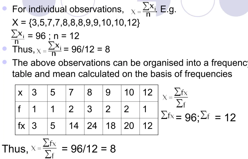
 _{For individual observations, . E.g.}

X = {3,5,7,7,8,8,8,9,9,10,10,12} = 96 ; n = 12

 Thus, = 96/12 = 8

 _{The above observations can be organised into a frequency}

table and mean calculated on the basis of frequencies

= 96; = 12

Thus, = 96/12 = 8

x 3 5 7 8 9 10 12

f 1 1 2 3 2 2 1

(13)

Central Tendency -

Mean

and

Mid-point

 Let say we have data like this:

Location Min Max

Town A 228 450

Town B 320 430

Price (RM ‘000/unit) of Shop Houses in Skudai

(14)

Central Tendency -

Mean

and

Mid-point

(contd.)



Let’s calculate:

Town A: (228+450)/2 = 339

Town B: (320+430)/2 = 375



Are these figures means?

(15)

Central Tendency -

Mean

and

Mid-point

(contd.)

 Let’s say we have price data as follows:

Town A: 228, 295, 310, 420, 450 Town B: 320, 295, 310, 400, 430

 Calculate the means?

Town A: Town B:

 Are the results same as previously?

(16)

Central Tendency – Mean of

Grouped Data

 House rental or prices in the PMR are frequently

tabulated as a range of values. E.g.

 What is the mean rental across the areas?

= 23; = 3317.5

Thus, = 3317.5/23 = 144.24

Rental (RM/month) 135-140 140-145 145-150 150-155 155-160

Mid-point value (x) 137.5 142.5 147.5 152.5 157.5

Number of Taman (f) 5 9 6 2 1

(17)

Central Tendency –

Median

 _{Let say house rentals in a particular town are tabulated:}

 _{Calculation of “median” rental needs a graphical aids→}

Rental (RM/month) 130-135 135-140 140-145 155-50 150-155

Number of Taman (f) 3 5 9 6 2

Rental (RM/month) >135 > 140 > 145 > 150 > 155

Cumulative frequency 3 8 17 23 25

1. Median = (n+1)/2 = (25+1)/2 =13th_.

Taman

2. (i.e. between 10 – 15 points on the vertical axis of ogive).

3. Corresponds to RM

140-145/month on the horizontal axis

4. There are (17-8) = 9 Taman in the range of RM 140-145/month

5. Taman 13th_{. is 5}th_{. out of the 9}

Taman

6. The rental interval width is 5

7. Therefore, the median rental can

be calculated as:

(18)

(19)

Central Tendency –

Quartiles

(contd.)

Upper quartile = ¾(n+1) = 19.5th_.

Taman

UQ = 145 + (3/7 x 5) = RM 147.1/ month

Lower quartile = (n+1)/4 = 26/4 = 6.5 th. Taman

LQ = 135 + (3.5/5 x 5) = RM138.5/month

Inter-quartile = UQ – LQ = 147.1 – 138.5 = 8.6th_{. Taman}

IQ = 138.5 + (4/5 x 5) = RM 142.5/month

(20)

Variability

 Indicates dispersion, spread, variation, deviation

 For single population or sample data:

where σ2_{and s}2_{= population and sample variance respectively, x} i = individual observations, μ = population mean, = sample mean, and n = total number of individual observations.

(21)

Variability (contd.)

 _{Why “measure of dispersion” important?}

 Consider yields of two plant species:

* Plant A (ton) = {1.8, 1.9, 2.0, 2.1, 3.6} * Plant B (ton) = {1.0, 1.5, 2.0, 3.0, 3.9}

Mean A = mean B = 2.28% But, different variability!

Var(A) = 0.557, Var(B) = 1.367

(22)

Variability (contd.)

 Coefficient of variation – CV – std. deviation as % of

the mean:

 A better measure compared to std. dev. in case

where samples have different means. E.g.

(23)

Spatial Statistics: Topic 3 23 Farm No. Yield (ton/ha) Species X Species Y

1 1.2 1.4

2 1.4 1.5

3 2.6 2.1

4 2.7 3.2

5 3.9 3.9

Mean 2.36 2.42

Var. 1.20 1.20

Variability (cont.)

Calculate CV for both species.

CV_x = (1.2/2.36) x 100

= 50.97%

CV_y = (1.2/2.42) x 100

= 49.46%

 Species X is a little more

(24)

Variability (cont.)

 Std. dev. of a frequency distribution

(25)

Probability distribution

 If there 20 lecturers, the probability that

A becomes a professor is: p = 1/20 = 0.05

 Out of 100 births, half of them were

girls (p=0.5), as the number increased to 1,000, two-third

were girls (p=0.67) but from a record of 10,000 new-born

babies, three-quarter were girls (p=0.75)

 The probability of a drug addict

recovering from addiction is 50:50

 General rule:

No. of times event X occurs Pr (event X) = Total number of occurrences

 Probability of certain event X to occur has a specific form of

distribution

Logical probability:

Experiential probability:

(26)

Probability Distribution

Dice1

Dice2 1 2 3 4 5 6

1 2 3 4 5 6 7

2 3 4 5 6 7 8

3 4 5 6 7 8 9

4 5 6 7 8 9 10

5 6 7 8 9 10 11

6 7 8 9 10 11 12

(27)

Probability Distribution (contd.)

Values of x are discrete (discontinuous)

Sum of lengths of vertical bars p(X=x) = 1

all x

(28)

Probability Distribution (cont.)

Age Freq Prob.

36 3 0.02

37 14 0.07

38 10 0.04

39 36 0.18

40 73 0.36

41 27 0.14

42 20 0.10

43 17 0.09

Total 200 1.00

Pr (Area under curve) = 1

Continuous variable

Mean = 39.5

(29)

 _{Pr (Age ≤ 36) =}_0.02

 _{Pr (Age ≤ 37) = Pr (Age ≤ 36) + Pr (Age = 37) = 0.02 + 0.07 =}_0.09

Probability Distribution (cont.)



Cumulative probability corresponds to the

(30)

 As larger and larger

samples are drawn, the probability distribution is getting smoother

 Tens of different types of

probability distribution: Z, t, F, gamma, etc

 Most important: normal

Larger sample

Very large sample

(31)

Normal Distribution - ND

 Salient features of ND:

* Bell-shaped, symmetrical * Total area under curve = 1 * Area under curve between any two points = prob. of

values in that range (shaded area) * Prob. of any exact value = 0

* Has a function of:

(32)

Normal Distribution - ND

Population 1 Population 2



₁



₂



₁



2

* A larger population has

narrower base (smaller *  determines location

(33)

Normal Distribution (cont.)

* Has a mean  and a variance 2, i.e. X  N(,



2 )

* Has the following distribution of observation:

“Home-buyers example…”

Mean age = 39.3

(34)

Standard Normal Distribution (SND)

 Since different populations have different  and 

(thus, locations and shapes of distribution), they have to be standardised.

 _{Most common standardisation: standard normal}

distribution (SND) or called Z-distribution

 _{(X=x) is given by area under curve}

 _{Has no standard algebraic method of integration}

→ Z ~ N(0,1)

 To transform f(x) into f(z):

x - µ

(35)

Z-Distribution

 _{Probability is such a way that:}

* Approx. 68% -1< z <1

(36)

Z-distribution (cont.)

 When X= μ, Z = 0, i.e.

 _{When X = μ + σ, Z = 1}

 When X = μ + 2σ, Z = 2

 When X = μ + 3σ, Z = 3 and so on.

 It can be proven that P(X₁ <X< X_k) = P(Z₁ <Z< Z_k)

 _{SND shows the}_{probability to the right}_{of any}

(37)

Normal distribution…Questions

A study found that the mean age, A of second-home buyers in Johor Bahru is 39.3 years old with a variance of RM 2.45.Assuming normality, how sure are you that the mean age is: (a) ≥ 40 years old; (b) 39 to 42 years old?

Answer (a): P(A ≥ 40)

= P[Z ≥ (40 – 39.3)/2.4] = P(Z ≥ 0.2917 0.3000) = 0.3821

(b) P(39 ≤ A ≤ 42)

= P(A ≥ 39) – P(A ≥ 42)

= 0.45224 – P[A ≥ (42-39.3)/2.4]

= 0.45224 – P(A ≥ 1.125) = 0.45224 – 0.12924

= 0.3230

Always remember: to convert to SND, subtract the mean and divide by the std. dev.

(38)

“Student’s t-Distribution”

 Similar to Z-distribution (bell-shaped, symmetrical)

 Has a function of

where  = gamma distribution; v = n-1 = d.o.f;  = 3.147

 Flatter with thicker tails

 _{Distributed with t}_{(0,σ) and -∞ < t < +∞}

 As _n→∞t(0,σ) → N(0,1)

 Probability calculation requires

(39)

How Are t-dist. and Z-dist. Related?



Using central limit theorem, N(, 2/n) will become

zN(0, 1) as n→∞

 For a large sample, t-dist. of a variable or a

parameter is given by:

The interval of critical values for variable, x is:

(40)

Skewness, m

₃

& Kurtosis, m

₄

 _{Skewness, m}

3 measures

degree of symmetry of distribution

 _{Kurtosis, m}

4 measures its

degree of peakness

 Both are useful when

comparing sample

distributions with different shapes

 Useful in data analysis

X_i = indivudal sample observation, =

(41)

Skewness

Bimodal Uniform J-shaped

Perfectly normal (zero skew) Right (+ve) skew Left (-ve) skew

  _

(42)

Kurtosis

Mesokurtic

(normal)

(zero kurtosis) Leptokurtic

(high peak)

(+ve kurtosis)

Platykurtic

(low peak)

(-ve kurtosis)

Mesokurtic distribution…kurtosis = 3

(43)

Spatial Statistics: Topic 3 43 X-coord. (000) Y-coord. (000) Trees with Ganoderma

535.60 104.80 8

536.70 107.30 12

536.80 106.80 11

537.30 107.31 12

537.15 105.40 13

537.40 105.37 13

538.48 107.82 9

542.22 106.10 8

540.35 105.91 7

540.10 104.95 7

540.30 104.75 6

538.75 102.80 5

545.10 105.90 4

546.30 105.90 3

547.15 105.90 2

Occurrence of ganoderma

X-coord. (000) Y-coord. (000) Trees with ganoderma

547.75 106.08 5

547.10 105.25 8

547.80 101.05 7

548.18 105.92 8

548.80 105.90 12

548.95 104.85 15

548.94 104.50 13

548.75 103.73 7

548.94 102.80 4

(44)

Al p.p.m. Freq. 0 0 250 7 500 13 750 25 1000 18 1250 13 1500 9 1750 7 2000 3 2250 4

E.g. Al₂++ + H

2++O--

→

Al₂O + H₂

sum 102.00

mean 1073.53

 553.05

 _305867.94

 169161266 .28  935551939 11.64 skew 0.77

(45)

E.g. W_CM = ((545.10-542.86)2 + (105.90-105.48)2)0.5

= (5.0176 + 0.1764)0.5

= 2.28 (i.e. 2,280 m)

Measures of spatial separation

Weighted mean centre (X_coord.) =

Weighted mean centre (Y_coord.) =

Standard distance =

(46)

Occurrence of ganoderma

Sum f = 191.00 Xw = 103687.00 Yw = 20147.40 (Xw- )2 =588.46 (Yw- )2 = 55.50

Weighted mean centre 542.86 105.48 Standard distance 1.84

Point to point distance (e.g.)

(47)

Spatial distribution – point data

(48)

Ethnic distribution of residence

k = (fx) -1

-8.15 t_c 0.12 _CV 0.02 CV 0.01 2 0.49 1.54 68 140  1.51 18 9 2 0.51 50 50 1 -0.49 0 81 0

(x- )2

fx f

x

H_o: 2_{= (pattern is random)}

H₁: 2_{> (pattern is clustered) or}2_{< (pattern is scattered)}

X = no. of observations per quadrat; f = frequency of quadrats; = (fx)/f; 2₌_{(x- )}2_/_{(fx) -1; CV =}2_{/ ;}

Reject Ho…

Descriptive statistics.