ABSTRACT
ROY, ARKAPRAVA. Bayesian Methods for High Dimensional Models in Brain Imaging. (Under the direction of Subhashis Ghoshal and Ana-Maria Staicu.)
In this thesis, we have worked on several methodology developments with the focus on brain imaging data. There is a general introduction to the materials covered in this thesis in Chapter 1.
In Chapter 2, we study possible relations between the structure of the connectome, white matter connecting different regions of brain and Alzheimer disease. Regression models in covari-ates including age, gender, and disease status for the extent of white matter connecting each pair of regions of the brain are proposed. Subject inhomogeneity is also incorporated in the model through random effects with an unknown distribution. Due to a large number of pairs of regions, we also adopt a dimension reduction technique through graphon (Lovasz and Szegedy (2006)) functions reducing functions of pairs of regions to functions of regions. The connecting graphon functions are considered unknown but assumed smoothness allows putting priors of low complexity on them. We pursue a nonparametric Bayesian approach by assigning a Dirich-let process scale mixture of zero mean normal prior on the distributions of the random effects and finite random series of tensor products of B-splines priors on the underlying graphon func-tions. Presence of interaction between region effects with covariates with sparsity restrictions is allowed in the model. Posterior computation techniques are developed. Posterior consistency of the proposed Bayesian approach is established under the asymptotic regime of increasing number of subjects and a fixed number of brain regions. Performance of the proposed Bayesian method is compared with ANCOVA models through simulations under both well-specified and misspecified cases. The proposed Bayesian approach is applied to a dataset obtained from ADNI consisting of 100 subjects and 83 brain regions. Bayes estimates of connectome strengths for a person with a given profile are obtained which can be used as a benchmark for the actual connectome data of a future patient with the same profile.
linear model with lasso penalization on the high dimensional covariate. The proposed Bayesian method is applied to a dataset of 748 individuals with 620,901 SNP and 8 other covariates for each individual.
Bayesian Methods for High Dimensional Models in Brain Imaging
by Arkaprava Roy
A dissertation submitted to the Graduate Faculty of North Carolina State University
in partial fulfillment of the requirements for the Degree of
Doctor of Philosophy
Statistics
Raleigh, North Carolina 2018
APPROVED BY:
Soumendra Nath Lahiri Brian J. Reich
Subhashis Ghoshal Co-chair of Advisory Committee
Ana-Maria Staicu
DEDICATION
BIOGRAPHY
ACKNOWLEDGEMENTS
I would like to extend my gratitude towards my advisors Dr. Subhashis Ghoshal and Dr. Ana Maria Staicu for giving exposure and guidance to lay the foundation for my research career. Their vast experience has helped me to finish my research works smoothly. I would like to thank Dr. Brian Reich for being part of the advisory committee as well as mentoring one of the research works of my thesis and also Dr. Soumendra Nath Lahiri and Dr. Ralph Smith to be part of the advisory committee and giving helpful comments on my work.
I met great people in this statistics department at North Carolina State University. All the support staffs have been extremely helpful so that everything went smoothly. I would like to thank Dr. Howard Bondel, Lanakila Alexander and Dr. Wenbin Lu for their help in any official issues as well as Terry Byron and Chris Waddell for any computing issues that I came across during my time here in the department. The computing facility in our department is not very best. But computing liaisons helped us at every stage. Also, I would like to thank the office of international students (OIS) for their help in any bureaucratic issues.
These four years have definitely been one of the best four years of my life. My stay at the USA has been very smooth. I am very fortunate to find a family with a wonderful group of friends including Sayan Banerjee, Sapna Rao, Suman Chakraborty, Sujatro Chakladar, Mityl Biswas, Priyam Das, Debraj Das, Arnab Hazra, Indranil Sahoo, Moumita Chakraborty, Sohini Raha, Arkopal Choudhury, Arnab Chakraborty, Suman Majumdar, Rahul Ghoshal, Dhrobo-jyoti Ghosh, Salil Konar, Aniket Bera, Abhishek Banerjee, Sayak Mukherjee, Abhra Sarkar, Rimli Sengupta, Jyotiska Dutta and Shalini Choudhury.
4.3.1 Image-on-image regression . . . 77
4.3.2 Scalar-on-image regression . . . 78
4.4 Computational details . . . 78
4.4.1 The model in spectral domain . . . 78
4.4.2 Imputation method . . . 79
4.4.3 Sampling . . . 81
4.5 Simulation results . . . 82
4.5.1 Image-on-scalar regression . . . 82
4.5.2 Image-on-image regression . . . 83
4.5.3 scalar-on-image regression . . . 87
4.6 Application to longitudinal MRI data . . . 93
4.7 Conclusion and discussion . . . 94
4.8 Proofs . . . 94
LIST OF TABLES
Table 2.1 Comparison of estimation accuracy for n= 500 in well-specified case . . . 18
Table 2.2 Comparison of estimation accuracy for n= 500 in misspecified case . . . 23
Table 2.3 Demographic table . . . 23
Table 3.1 For non-linear case . . . 48
Table 3.2 For linear case . . . 48
Table 3.3 Demographic table . . . 58
Table 3.4 Estimates of covariates for Total Brain for slope from non-linear model . . . . 60
Table 3.5 Estimates for Ventricles for slope . . . 60
Table 3.6 Estimates for Left Hippocampus for slope . . . 61
Table 3.7 Estimates for Right Hippocampus for slope . . . 61
Table 3.8 Estimates for Left inferior lateral ventricle for slope . . . 62
Table 3.9 Estimates for Right inferior lateral ventricle for slope . . . 62
Table 3.10 Estimates for Left Medial Temporal for slope . . . 63
Table 3.11 Estimates for Right Medial Temporal for slope . . . 63
Table 3.12 Estimates for Left Inferior Temporal for slope . . . 64
Table 3.13 Estimates for Right Inferior Temporal for slope . . . 64
Table 3.14 Estimates for Left Fusiform for slope . . . 65
Table 3.15 Estimates for Right Fusiform for slope . . . 65
Table 3.16 Estimates for Left Entorhin for slope . . . 66
Table 3.17 Estimates for Right Entorhin for slope . . . 66
Table 3.18 Estimates of covariates for Total Brain for slope from linear model . . . 67
Table 3.19 SNPs selected after variable selection from non-linear model along with gene names and main effect on slope . . . 67
Table 4.1 Total MSE, MSE for the subregion with trueβ = 0 along with standard errors in the bracket, power, coverage and Type 1 error for the slope of the image-on-scalar simulation with different SNRs for Gaussian, PING 3 and PING 5 as choices of prior . . . 85
Table 4.2 Total MSE, MSE for the subregion with trueβ = 0 along with standard errors in the bracket, power, coverage and Type1 error for the slope of the image-on-image simulation with different SNRs for Gaussian, PING 3 and PING 5 as choices of prior . . . 88
Table 4.3 Total MSE, MSE for the subregion with trueβ = 0 along with standard errors in the bracket, power, coverage and Type1 error for the slope of the scalar-on-image regression model with different true variances for Gaussian, PING 3 and PING 5 as choices of prior . . . 91
LIST OF FIGURES
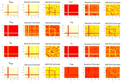
Figure 2.1 Heatmap of number in log-scale and average width of white matter fibers where each pixel represents each pair of region. . . 7 Figure 2.2 Heatmap of truth along with Bayesian methods and ANCOVA estimates for
sample size 500 in the well specified case with 20 nodes. . . 19 Figure 2.3 Plot of squared bias and variance for different parameters against sample
sizes for Bayesian method and ANCOVA estimates in the well-specified case. 20 Figure 2.4 Heatmap of truth along with Bayesian methods and ANCOVA estimates for
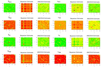
sample size 500 in the misspecified case with 20 nodes. . . 21 Figure 2.5 Plot of squared bias and variance for different parameters against sample
sizes for Bayesian method and ANCOVA estimates in the misspecified case. . 22 Figure 2.6 Effect of different covariates on connection width, each circle denotes
differ-ent cortical brain regions and edge-widths are proportional to the degree of significance of that edge. . . 24 Figure 2.7 Effect of covariates on connection-probability, each circle denotes different
cortical brain regions and edge-widths are proportional to the degree of sig-nificance of that edge. . . 25 Figure 2.8 Effect of covariates on number of connections, each circle denotes different
cortical brain regions and edge-widths are proportional to the degree of sig-nificance of that edge. . . 26 Figure 3.1 Anatomic parcellation of cortical surface from different angles showing brain
regions used for analysis. . . 38 Figure 3.2 Spike distribution withM1 = 0.01 andM2 = 10. . . 43
Figure 4.1 Comparison of Gaussian density with PING-3 and PING-5 densities. . . 75 Figure 4.2 Conditional density plot of β2 given different values of β1 for different
corre-lations and components for bivariate realization (β1, β2) at two locations. . . 76
Figure 4.3 3-D image of the true slopeβ(s) for the image-on-scalar regression simulation study. . . 84 Figure 4.4 Plot of the estimates for the slope of the image-on-scalar regression
simu-lation with different signal to noise ratios (SNRs) for Gaussian, Product of independent Gaussian with 3 components (PING 3) and PING 5 as choices of prior. . . 86 Figure 4.5 Plots of the truth for last five regression coefficients (first five were zero) from
second simulation corresponding to image-on-image regression. . . 87 Figure 4.6 Comparison plot of the estimates for the slope of the scalar-on-image
sim-ulation with different true variances for Gaussian, PING 3 and PING 5 as choices of prior. . . 90 Figure 4.7 Variation in MSE of estimated slope for varying number of componentsq for
scalar-on-image simulation. . . 92 Figure 4.8 Data for each visit of the middle slice of the MRI image for 12 visits of the
LIST OF SYMBOLS
((A))i,j : a matrix A with (i, j)th element being Ai,j.
AT : transpose of the matrixA.
Ai,: the ith row ofA.
A,j : thejth column of A.
vec(A) : the vector obtained by stacking the columns of the matrix A one over another.
A⊗B : the Kronecker product betweenA and B.
Ip : the identity matrix of orderp.
maxeig(A) : the maximum eigenvalue of the matrix A. mineig(A) : the minimum eigenvalue of the matrix A. kxk: Pp
i=1x2i
1/2
, theL2 norm of the vector x.
a·b: element wise product of two vectors aand b. l
1A(·) : indicator function of the setA.
an=o(bn) : an/bn→0 as n→ ∞ for numerical sequencesan andbn.
an=O(bn) : an/bn is bounded.
anbn:an=O(bn) andbn=O(an).
an.bn:an=O(bn).
anbn:bn=o(an).
anbn:an=o(bn).
oP(1) : a sequence of random variables which converges in probability to zero.
OP(1) : a sequence of random variables bounded in probability.
E(·) : the mean vector of a random vector.
Var(·) : the dispersion matrix of a random vector. dH(P, Q) =
q R
(√p−√q)2, the Hellinger distance between P and Q.
K(p, q) =Plogpq, the Kullback-Leibler distance betweenP andQ. L: class of real-valued smooth continuous functions on [0,1]2. a∧b: the minimum of two real numbers aand b.
|r|:Ps
Chapter 1
Introduction
Developing methodologies for high dimensional datasets are new challenges in the field of statis-tics. There are many sources of occurrences of such datasets like genomics, neuroscience, finance, earth sciences etc. We apply our methods to brain image data. Thus our methods are mostly motivated by application in brain imaging data but can be useful for other kinds of high di-mensional datasets as well.
There are different kinds of neurological datasets available currently. There are data of structural brain, human brain connectome, magnetic resonance imaging (MRI) data, functional magnetic resonance imaging (fMRI) data etc. Some diseases are known to affect the human brain. The motivation to study these datasets is to understand the direct or indirect effect of these diseases on the human brain. Potentially there are three kinds of brain image datasets, namely brain connectome, brain anatomy and neuronal signal images.
The brain connectome is a comprehensive map of all the neural connection within the brain. It is very difficult to construct the connectome from the MRI images. Several researchers are using these connectome datasets to answer various kinds of questions. There are many scientific questions that the researchers are trying to answer as well several novel statistical methodologies are being developed for these complex network datasets. This kind of data is used to study diseases with the neurodegenerative disorder like Parkinson disease, Alzheimer disease etc. In this thesis, we focus on the studying brain connectome in connection with Alzheimer disease.
to amyloid plaque burden, which is one of the pathological hallmarks of AD and has been shown to become elevated years before the onset of clinical symptoms (Prescott et al. (2014)). It may be that these structural connections are part of the anatomic substrate underlying cognition. In Chapter 2 of this thesis, we model changes in the brain connectome caused by the onset of the disease using a graphical structure.
Studying brain anatomy and its changes over time in a healthy or a disease patients are also some interesting works that researcher from various domains is interested in. One such issue is with brain atrophy. The shape and size of the brain change with time and these variations change across individuals. In Chapter 3 we study this problem. It is believed to have a prolonged preclinical phase initially characterized by the development of silent pathologic changes when patients appear to be clinically normal, followed by mild cognitive impairment (MCI) and then dementia (AD) (Petrella (2013)). Apart from its manifestation in the impairment of cognitive abilities, disease progression also produces a number of structural changes in the human brain, which includes the deposition of amyloid protein and the shrinkage or atrophy for certain regions of the brain over time (Thompson et al. (2003)). Previous studies have shown that the rate of brain atrophy is significantly modulated by a number of factors, such as gender, age, baseline cognitive status and most markedly, allelic variants in the APOE gene (Hostage et al. (2014)). In this paper, we examine if any other genes are also implicated in modulating the rate of brain atrophy. This analysis represents a technical challenge because the genomic data is high dimensional and needs to be incorporated into a model for longitudinal progression of brain volumes measured in multiple parts of the brain. We examine the effects of age, gender, APOE genes, genetic variation and Alzheimer disease on atrophy of the brain regions. To summarize the effects of the said covariates a nonparametric single model is proposed with two separate inputs for high dimensional and low dimensional covariates separately. We develop a Bayesian estimation procedure to get the estimates of the model parameters. The proposed Bayesian method is applied to a dataset of 748 individuals with 620,901 SNP and 8 other covariates for each individual.
be continuous, sparse and piecewise smooth.
Chapter 2
Bayesian Modeling of the Structural
Connectome for Studying Alzheimer
Disease
This chapter’s material is a joint work with Subhashis Ghosal, Jeffrey Prescott and Kingshuk Roy Choudhury.
2.1
Introduction
Our study is performed using data obtained by Alzheimer Disease Neuroimaging Initiative (ADNI − adni.loni.usc.edu). Using T1-weighted magnetic resonance (MR) images from ADNI, the cortex of the brain is divided into several regions using a standard anatomic atlas. These regions are connected by white matter fibers, identified using diffusion tensor imaging (DTI) MR. The graphical representation of these white matter connections between cortical regions is referred to as the connectome. It is thought that some of these connections between brain regions become weakened over time due to the AD. Some other factors like age or sex might also affect this connectome, as well as subject-specific random effects. We model the connectome using graph theoretic metrics, accounting for patients specifics effects and implement a Bayesian analysis.
of white matter fiber and the mean width of white matter fibers between them when at least a connecting white matter fiber exists. Our aim is to identify the pairs of regions between which the connections are affected by the disease and other covariates differently than in other pairs in the connectome by the covariates. The aspects of the presence of a connection, the number of connections and the mean width are modeled respectively by a binary regression model with a probit link, a Poisson regression model with an exponential link and a normal regression model. Interactions of covariates with pairs of regions are considered, but a sparsity condition is imposed in the analysis through the prior, which imply that for most pairs, these effects are the same and possibly non-zero while for a few of pairs, there could be different effects. In fact, detecting such region-pairs is the main objective of our analysis. Because the number of region-pairs is prohibitively high, it leads to a very high dimensional regression model if a naive approach is taken. Hence we use a dimension reduction technique that introduces a latent variable for each region and expresses functions of region-pairs in terms of a single smooth unknown function of each pair of latent variables as in a graphon model (Lovasz and Szegedy (2006)). If (ajk : j, k = 1, . . . , J) is an array of parameters, then we model ajk = g(uj, uk),
where u1, . . . , uJ are latent variables and g is a function of two arguments. Symmetry of the
matrix ((ajk)) is respected if g is symmetric in its arguments. The original motivation for this
representation is that if ajk, j, k = 1, . . . , J are random variables such that the matrix ((ajk))
is distributionally invariant under permutations of rows and columns, thenajk =g(uj, uk) for
some latent variables u1, . . . , uJ that can be assumed to be uniformly distributed and a
func-tion g called a graphon function. In the present context, if the parameters ajk, j, k= 1, . . . , J
are treated as random, then such row and column wise exchangeability conditions are natural non-informativeness conditions. Given the graphon function, thus the strength of connections is determined by only 83 latent variables linked with each region instead of being 832
typically show more pronounced effects. This feature can be captured by a prior which intro-duces sparsity in the coefficients by making most of the latent variables cluster at a point with high probability. To reduce additional computational burden arising out of selection of active latent variables which do not cluster at the benchmark point, we use a continuous shrinkage prior instead of more traditional point mass spike and slab prior such as the horseshoe prior (Carvalho et al. (2010)), normal-gamma prior (Griffin and Brown (2010)), double-Pareto prior (Armagan et al. (2013)) or Dirichlet-Laplace prior (Bhattacharya et al. (2015)).
The rest of the chapter is organized as follows. In the next section, we describe the details of modeling the connectome dataset from ADNI. In Section 2.3, we describe the prior construc-tion and develop posterior computing techniques. A simulaconstruc-tion study comparing the proposed Bayesian procedure with ANCOVA-based ones is conducted in Section 2.4. The real data on connectome from ADNI is analyzed in Section 2.5. We study the posterior consistency of the proposed Bayesian procedure in Section 2.6 under the asymptotic regime that the number of subjects is going to infinity but the number of regions is remaining fixed. The result justifies the use of the proposed Bayesian procedure also from a frequentist perspective. Proof of the posterior consistency result is given in the Section 2.6.1.
2.2
Data description and modeling
In the ADNI dataset on connectome, the brain is divided into J = 83 regions. For each pair of brain regions, the number of white matter fibers between them and their average widths are obtained.
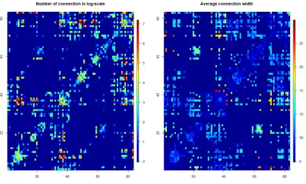
The data is obtained forn= 100 subjects, for whom information regarding disease prognosis, sex and age are obtained. For many edges in Figure 2.1, the mean widths are not defined where there are no white matter fibers. There are three disease prognosis states, Alzheimer (AD), mild cognitive impairment (MCI) and no cognitive impairment (NC). There may not be any white matter fiber connecting two brain regions for some subjects.
Except for age, the other two covariates, sex and disease prognosis, are categorical. Since disease prognosis has three possible states, we introduce dummy variables ZMCI and ZAD respectively standing for the onset of MCI and AD, setting NC at the baseline. Similarly, the dummy variable ZM indicating male gender is introduced setting females at the baseline. Let Z = (ZMCI, ZAD, ZM,Age)0 stand for the whole vector of covariates and Zi stand for its value
for theith subject. LetNijkstand for the number of white matter fiber connecting brain regions
j and k in the ith subject, and Wijk the mean width of such fibers, provided that Nijk ≥ 1.
In ADNI dataset, there were no missing values in Nijk or Wijk. Some of the covariates were
Figure 2.1: Heatmap of number in log-scale and average width of white matter fibers where each pixel represents each pair of region.
all subjects.
It seems natural to consider a Poisson model for the counts of fibers connecting two regions in a subject. However, as shown in Figure 2.1, the abundance of zero connections makes the Poisson model somewhat inappropriate. We overcome the problem by considering a zero-inflated Poisson model, by boosting the probability of zero through a binary latent variable Ξijk with
parameter Φ(πijk), where Φ stands for the standard normal distribution function andπijk is a
real-valued parameter. If Ξijk = 0, then Nijk is set at zero, while if Ξijk = 1, the number of
connectionsNijkis assumed to be Poisson distributed with some positive meaneλijk. Note that
in our formulation Ξijk is not completely identifiable since the value Nijk = 0 is compatible
with both possible values of Ξijk. If Nijk ≥ 1, we assume that the mean fiber width, in the
logarithmic scale, is normally distributed with some meanµijk, and variance σ2/Nijk for some
unknown σ > 0. The heuristic justification of the choice of the variance σ2/Nijk stems from
fiber widths are positive, the model seems to fit the data better in the logarithmic scale, and the heuristics for the choice of the variance extends to the logarithmic scale by the delta method, at least whenNijk is large. Thus we can represent the data generating process as
Ξijk∼Bin(1,Φ(πijk))
Nijk|{Ξijk= 1} ∼Poisson(eλijk) (2.1)
logWijk=µijk+ijk, ijk|{Nijk ≥1} ∼N(0, σ2/Nijk).
A simple analysis of covariance (ANCOVA)-type model can be formulated to describe linear effects of the covarites Zi on each unrestricted parameter πijk, λijk and µijk for each pair of
brain regions (j, k):
µijk= ((µ0))j,k+Zi0χjk +η1i,
πijk = ((π0))j,k+Zi0βjk +η2i, (2.2)
λijk= ((λ0))j,k+Zi0νjk+η3i,
where ((µ0))j,k, ((π0))j,k and ((λ0))j,k are baseline values of µijk, πijk and λijk respectively for
covariate valueZi= 0.
χjk = (((χMCI))j,k,((χAD))j,k,((χM))j,k,((χAge))j,k)0,
βjk = (((βMCI))j,k,((βAD))j,k,((βM))j,k,((βAge))j,k)0, (2.3)
νjk = (((νMCI))j,k,((νAD))j,k,((νM))j,k,((νAge))j,k)0
are regression coefficients for the average width, connection probability and number of con-nections respectively and ((.))j,k denotes (j, k)th element of a matrix, and ηi = (η1i, η2i, η3i)0,
i= 1, . . . , n, are independent random effects of theith subject distributed according to an un-known common distribution. It may be noted that the normal distribution function Φ and the exponential function are used respectively as link functions for binary and Poisson regression. For the latter, the exponential link is almost a universal choice, while for binary regression both logistic and probit (i.e. Φ) links are commonly used and usually give similar results. Our pref-erence for the probit link is due to its computational advantage in a Gibbs sampling scheme for Bayesian computation, through a data-augmentation technique (see Albert and Chib (1993)).
For a preliminary analysis, we fit the model using a generalized heteroscedastic ANCOVA, ignoring the zero-inflation aspect and the random effects in the model.
The model thus has 3× 832
method failed to give estimates of either µ0,jk orχjk. For the Poisson regression, theglm
func-tion in R did not converge for several pairs (j, k). This suggests using a dimension reducfunc-tion of the parameter space through further modeling if we want to conduct an edge-wise analysis. The dimension reduction also helps with computation and gives easy interpretability of the results. Since the parameters are indexed by edges, a substantial reduction of dimension will be possible if these can be viewed as arising from some latent characteristics of nodes through some fixed but unknown function. This can be motivated from exchangeability considerations. In the absence of initial information about connections between regions, exchangeability seems to be an appealing assumption. By a well known representation theorem of exchangeable random graphs (c.f. Aldous (1981), Hoover (1979)), a function of edge (j, k) can then be represented as f(ξi, ξj) whereξi, for each nodeiis a latent variable independently and identically distributed
and f is a fixed function, called a graphon, irrespective of the size of the network. Assuming that the function f is sufficiently smooth, a basis expansion can approximate it using only fewer terms. Thus the graphon technique in our context will be able to reduce a parameter array of size 832
= 3486 to only a parameter vector of size 83 +K, where K is the number of parameters used to approximate the unknown smooth graphon function. Typically a modest number of terms suffices for well-behaved functions using standard bases such as B-splines or polynomials. As a result, a substantial dimension reduction is possible through the graphon technique. This leads to modeling the arrays of baseline values and regression coefficient as
((µ0))j,k =µ(ξj, ξk), ((π0))j,k =π(ξj, ξk), ((λ0))j,k =λ(ξj, ξk),
((χl))j,k =χl(δj, δk), l= MCI, AD, M, Age, (2.4)
((βl))j,k =βl(δj, δk), l= MCI, AD, M, Age,
((νl))j,k =νl(δj, δk), l= MCI, AD, M, Age,
where, with an abuse of notations, µ,π,λ, χMCI,χAD, χM,χAge,βMCI,βAD,βM,βAge,λMCI,
λAD, λM and λAge are smooth functions on the unit square [0,1]2 and symmetric in their
arguments, andξ1, . . . , ξJ and δ1, . . . , δJ are latent variables taking values in the unit interval.
The reason for choosing two separate sets of latent variables is to distinguish between fixed and sparse main effect.
2.3
Prior specification and posterior computation
2.3.1 Prior specification
To proceed with a nonparametric Bayesian analysis, we put prior distributions on the smooth functions appearing in the graphon representation through basis expansion in tensor products of B-splines, and on the coefficients of the basis expansion. The coefficients can be arranged in the form of a square matrix. The symmetry of the matrices of coefficients ensures symmetry of the resulting functions in its arguments as required by graphon functions. Given other set of parameters and values of the random effects, (independent) normal prior on the coefficients of the tensor products of B-splines will lead to conjugacy in the normal regression model for the width, allowing a simple and fast posterior updating rule. In the binary regression model for the connection probability, normal prior still leads to conjugacy using the data augmentation technique of Albert and Chib (1993). Since no conjugacy is possible for the Poisson regression for the number of connections, Metropolis-Hastings is applied. Alternatively, adaptive rejection sampling can be applied to obtain posterior updates. Thus a spike and slab density for the latent variables with a spike at 1/2 should be able to catch the desired sparsity. We however only induce approximate sparsity though a well-peaked symmetric beta density in place of a point mass at 1/2, which is computationally more convenient. On the distribution G of the random effects, we put a Dirichlet process scale mixture of zero mean normal prior (see Chapter 5 of Ghosal and van der Vaart (2017)).
More specifically, the prior can be completely described by the following set of relations: (i) Graphon functions:
µ(ξj, ξk) = K
X
m=1 K
X
m0=1
θ1,mm0Bm(ξj)Bm0(ξk),
π(ξj, ξk) = K
X
m=1 K
X
m0=1
θ2,mm0Bm(ξj)Bm0(ξk),
λ(ξj, ξk) = K
X
m=1 K
X
m0=1
and for l= MCI,AD,M,
χl(δj, δk) = K
X
m=1 K
X
m0=1
γ1l,mm0Bm(δj)Bm0(δk),
βl(δj, δk) = K
X
m=1 K
X
m0=1
γ2l,mm0Bm(δj)Bm0(δk),
νl(δj, δk) = K
X
m=1 K
X
m0=1
γ3l,mm0Bm(δj)Bm0(δk),
where θt,mm0 = θt,m0m for all t = 1,2,3, and γtl,mm0 = γt,m0m for all t = 1,2,3, l = MCI,AD,M, and that
(a) graphon coefficients: For some chosen a >0,
θt,mm0 ind∼ N(0, a2), γtl,mm0 ind∼ N(0, a2), 1≤m≤m0 ≤K, fort= 1,2,3,l= MCI,AD,M;
(b) latent variables: ξ1, . . . , ξJ
ind
∼ Un(0,1), δ1, . . . , δJ ind
∼ qUn(0,1) + (1−q)Be(M, M),
the mixing probabilityqis given a default uniform prior Un(0,1) andM >0 is chosen big; here Un stands for the uniform distribution and Be for the beta distribution. (ii) Random effects distribution: Fort= 1,2,3 andi= 1, . . . , n,
ηti|τti ind
∼ N(0, τti2), τti2 ind∼ Gt, t= 1,2,3, Gt ind
∼ DP(αtIG(b1, b2)),
where DP stands for the Dirichlet process, IG for the inverse-gamma distribution and the precision parameter αt of the Dirichlet process is given a gamma priorαt∼Ga(c1, c2).
2.3.2 Posterior updating
Introduce a latent variable Ij the indicator of the Un(0,1) component of the distribution ofδj,
j= 1, . . . , J. Now the log-likelihood is given by C−X
i,j,k
exp{X
m,m0
[θ3,mm0Bm(ξj)Bm0(ξk) + X
l
γ3l,mm0Bm(δj)Bm0(δk)Zil] +η3i}
+X
i,j,k
Nijk[
X
m,m
(θ3,mm0Bm(ξj)Bm0(ξk) + X
l
γ3l,mm0Bm(δj)Bm0(δk)Zil) +η3i]+
− 1 2σ2
X
i,j,k
Nijk[logWijk− K
X
m=1 K
X
m0=1
(θ1,mm0Bm(ξj)Bm0(ξk)
+X
l
γ1l,mm0Bm(δj)Bm0(δk)Zil) +η1i]2
+X
i,j,k
I(Nijk = 0) log Φ
X
m,m0
(θ2,mm0Bm(ξj)Bm0(ξk)
+ X
l
γ2l,mm0Bm(δj)Bm0(δk)Zil) +η2i
+X
i,j,k
(1−I(Nijk= 0)) log 1−Φ
X
m,m0
(θ2,mm0Bm(ξj)Bm0(ξk)
+X
l
γ2l,mm0Bm(δj)Bm0(δk)Zil) +η2i
− 1 2a2
X
m≤m0
(θ1,mm2 0+θ2,mm2 0+θ3,mm2 0)
− 1 2a2
X
m≤m0 X
l
(γ1,mm2 0l+γ2,mm2 0l+γ3,mm2 0l)
+ log (1−Ij)δjM−1(1−δj)M−1
Γ(M)2 Γ(2M)+Ij
+Ijlogq+ (1−Ij) log(1−q)−(nJ2/2 +d1−1) logσ2−d2/σ2,
where C involes only hyperparameters a, M, K, b1, b2, c1, c2, d1, d2, q and the observations, but
not the parameters of the model.
Posterior updates are explained here. For notational convenience we define θ1 = (θ1,mm0 : 1≤m≤m0 ≤K), γ1l= (γ1l,mm0 : 1≤m ≤m0 ≤K, l= MCI,AD,M), θ2 = (θ2,mm0 : 1≤m≤ m0 ≤K),γ2l= (γ2l,mm0 : 1≤m≤m0 ≤K, l= MCI,AD,M),θ3= (θ3,mm0 : 1≤m≤m0 ≤K), γ3l = (γ3l,mm0 : 1 ≤ m ≤ m0 ≤ K, l = MCI,AD,M), ξ = (ξ1, . . . , ξK), δ = (δ1, . . . , δK), (I1, . . . , IK), η1 = (η11, . . . , η1n), η2 = (η21, . . . , η2n), η3 = (η31, . . . , η3n), τ1 = (τ11, . . . , τ1n),
τ2 = (τ21, . . . , τ2n), τ3 = (τ31, . . . , τ3n), σ. Let A be a symmetric matrix of dimension K ×K,
of unique entries ofA. We can construct matrix B of dimension K2
×K such that vec(A)0 = uni(A)0B. Let ψjk = (Bm(ξj)Bn(ξk) : 1 ≤m≤m0 ≤K) andψ0jk = (Bm(δj)Bn(δk) : 1 ≤m≤
m0 ≤K). To perform data augmentation technique for block updating parameters in the probit regression part, we introduce latent variable Lijk. Here we use Idl to denote identity matrix of
dimensionl.
• Updating σ2: Generate a sample from the inverse gamma distribution with parame-ters (d1+nJ2/2) and d2+Pi,j,kNijk[logWijk−PKm=1
PK
m0=1(θ1,mm0Bm(ξj)Bm0(ξk) + P
lγ1l,mm0Bm(δj)Bm0(δk)Zil) +η1i]2.
• Updating θ1: Generate a sample from the multivariate normal distribution with mean
Mθ1 =Vθ1B(
P
i,j,kψjkNijk(logWijk−
P
lγ1lBψ
0
jk)) and varianceVθ1 =
(P
i,j,kNijkψjk)0(Pi,j,kNijkψjk)/σ2+ IdK(K+1)/2/a2
−1 .
• Updating γ1l: Generate a sample from the multivariate normal distribution with mean
Mγ1l = Vγ1lB(
P
i,j,kψjkNijk(logWijk −
P
v6=lγ1vBψ
0
jk −θ1Bψjk)) and variance Vγ1l =
(P
i,j,kNijkZilψjk0 )0(Pi,j,kNijkZilψ0jk)/σ2+ IdK(K+1)/2/a2
−1 ,Mγ1l
= Vγ1lB(
P
i,j,kψjkNijk(logWijk −Pv6=lγ1vBψjk0 −θ1Bψjk)). Generate γ1l from
Multi-variate normal with meanMγ1l and covariance matrixVγ1l
• Updating Lijk: The posterior distribution ofLijk is
N(X
m,m0
(θ2,mm0Bm(ξj)Bm0(ξk) + X
l
γ2l,mm0Bm(δj)Bm0(δk)Zil) +η2i,1),
truncated to [0,∞) if Nijk>0, but truncated to (−∞,0) ifNijk = 0.
• Updating θ2: Generate a sample from the multivariate normal distribution with mean
Mθ2 =Vθ2B(
P
i,j,kψjk(Lijk−
P
lγ2lBψjk0 )) and varianceVθ2 =
(P
j,knψjk)0(
P
j,knψjk)+
IdK(K+1)/2/a2−1 .
• Updating γ2l: Generate a sample from the multivariate normal distribution with mean
Mγ2l=Vγ2lB(
P
i,j,kψjk(Lijk−
P
v6=lγ2vBψ0jk−θ2Bψjk)) and varianceVγ2l =
(P
j,knZil2ψ
0
jk)
0(P
j,knZilψ
0
jk)/σ2+ IdK(K+1)/2/a2
−1 .
• Updating θ3,mm0: Execute the following steps of the Metropolis-Hastings algorithm: – generate3,mm0 from N(0, s3) for some suitably tuned s3 >0 (see below); – updateθ3,mm0 toθ∗
where logL(m, m0, x) is given by −X
i,j,k
exp{ X
v,v06=m,m0
[θ3,vv0Bv(ξj)Bv0(ξk)] + X
l,v,v0
γ3l,vv0Bv(δj)Bv0(δk)Zil] +xBm(ξj)Bm0(ξk) +η3i}
+X
i,j,k
Nijk[
X
v,v06=m,m0
(θ3,vv0Bv(ξj)Bv0(ξk) + X
l
γ3l,vv0Bm(δj)Bm0(δk)Zil) +xBm(ξj)Bm0(ξk) +η3i].
• Updating γ3l,mm0: Execute the following steps of the Metropolis-Hastings algorithm: – generate3l,mm0 from N(0, s3l) for some suitabley tuned s3l>0 (see below); – updateγ3l,mm0 toγ∗
3l,mm0 =γ3l,mm0+3l,mm0 with probability Pa,3l,mm0 = min
nL1(l, m, m0, γ3l,mm∗ 0) L1(l, m, m0, γ3l,mm0),1 , where logL1(l, m, m0, x) is given by
−X
i,j,k
exp{ X
v,v06=m,m0
[θ3,vv0Bt(ξj)Bt0(ξk) + X
l
γ3l,vv0Bv(δj)Bv0(δk)Zil] +xBm(δj)Bm0(δk) +θ3,mm0Bm(ξj)Bm0(ξk) +η3i}
+X
i,j,k
Nijk[
X
v,v06=m,m0
(θ3,vv0Bv(ξj)Bv0(ξk) +xBm(ξj)Bm0(ξk)
X
l
γ3l,vv0Bm(δj)Bm0(δk)Zil) +xBm(δj)Bm0(δk) +θ3,mm0Bm(ξj)Bm0(ξk) +η3i].
• Updating δj: Execute the follwing steps of the Metropolis-Hastings algorithm:
– generateU1j from Be(B1, B1);
– updateδj toδj∗ =δjU1j/{δjU1j+ (1−δj)(1−U1j)} with probability
Pa,δj = min
nL2(j, δj∗)f(δj|δ∗j) L2(j, δj)f(δj∗|δj)
,1o,
whereL2(j, x) denotes likelihood at δj =x (keeping other parameters fixed) and
f(δj∗|δj) =
( δj(1−δ ∗
j)
δj+δ∗j−2δjδ∗j)
B1−1(1− δj(1−δ
∗
j)
δj+δj∗−2δjδj∗)
B1−1
B(B1, B1)
δj∗(1−δj∗) (δj +δj∗−2δjδj∗)2
here B(a, b) = Γ(a)Γ(b)/Γ(a+b) is the beta function, and B1 > 0 is to be tuned
suitably (see below).
• Updating ξj: Execute the follwing steps of the Metropolis-Hastings algorithm:
– generateU2j from Be(B2, B2);
– updateξj toξj∗ =ξjU2j/{ξjU2j + (1−ξj)(1−U2j)}with probability
Pa,ξj = min
nL3(j, ξj∗)f2(ξj|ξj∗) L3(j, ξj)f2(ξj∗|ξj)
,1o,
whereL3(j, x) denotes likelihood at ξj =x (keeping other parameters fixed),
f(ξ∗j|ξj) =
( ξj(1−ξ ∗
j)
ξj+ξ∗j−2ξjξ∗j)
B2−1(1− ξj(1−ξ
∗
j)
ξj+ξj∗−2ξjξj∗)
B2−1
B(B2, B2)
ξj∗(1−ξj∗) (ξj+ξj∗−2ξjξj∗)2
;
and B2 >0 is to be tuned suitably (see below).
• Updating η1: Generate a sample from the multivariate normal distribution with mean
Mη1 =Vη1(κ11, . . . ,κln), where κ1i
=P
jkNi,j,k(logWijk−
PK
m=1
PK
m0=1(θi,mm0Bm(ξj)Bm0(ξk)+P
lγil,mm0Bm(δj)Bm0(δk)Zil)), i= 1, . . . , n, and covariance
Vη1 =
diag(X
jk
N1,j,k,· · · ,
X
jk
Nn,j,k)/σ2+ diag(1/τ112,· · ·,1/τ1n2 )
−1 .
• Updating η2: Generate a sample from the multivariate normal distribution with mean
Mη2 =Vη2(κ21, . . . ,κ2n), whereκ2i=
P
jk(Lijk−
PK
m=1
PK
m0=1(θ2,mm0Bm(ξj)Bm0(ξk) + P
lγ2l,mm0Bm(δj)Bm0(δk)Zil)), i = 1, . . . , n, and covariance
Vη2 =
diag(J2,· · ·, J2) + diag(1/τ212 ,· · · ,1/τ2n2 )−1 .
• Updating η3i: Execute the following steps of the Metropolis-Hastings algorithm:
– generate3,i from N(0, s3η) for some suitable tuneds3>0;
– updateη3i toη3i∗ =η3i+3,i with probability
Pa,3,η = min
L4(i, η∗3i)
L4(i, η3i)
where logL4(i, x) is given by
−X
j,k
exp{X
m,m0
[θ3,mm0Bm(ξj)Bm0(ξk)
+X
l
γ3l,mm0Bm(δj)Bm0(δk)Zil] +x}]}
+X
j,k
Nijk[
X
m,m
(θ3,mm0Bm(ξj)Bm0(ξk)
+X
l
γ3l,mm0Bm(δj)Bm0(δk)Zil) +x]−x2/(2τ3i2).
• Updating τti: Execute the following steps of the P`olya urn scheme:
– generater with P(r =l) =qt,il/{Pkqt,ik}, where
qt,ij∝
1
τtj exp(−η
2
ti/(2τtj2)), ifj6=i, j≥1
αt[τ−0.5−b1/2−1exp(
−η2
ti/2−b2
τ2
ti )], ifj=i;
– ifr=i, sample τti2 from Ga(−0.5−b1/2, η2ti/2 +b2), else set τti=τtr. • Updating ofq: Generateq from Be(P
jIj + 1, J −PjIj).
2.3.3 Tuning
In the above Metropolis-Hastings steps, we need to tunes3,s31,s32,s33,B1,B2 and s3η (these
are defined in the supplementary material) to achieve good acceptance rates. We automatically adjust those values after every 500 iterations. The standard deviations are reduced (respectively, increased) to increase (respectively, to reduce) the acceptance rate of the Metropolis-Hastings moves. On the other hand,B1 and B2 are increased (respectively, reduced) to increase
(respec-tively, to reduce) the acceptance rate of the corresponding parameters. IfUj = 0.5, update will
be same as the current value. So, the distribution ofUj should have a high concentration at 0.5
to make a local move from the current state. A higher value of B will induce a proposed move in the close vicinity of the original position while a smaller value will lead to a proposed move to a farther location. Tuning the values of B1 and B2 can help maintain a desirable proportion
2.4
Simulation
In this section, we study the performance of the proposed Bayesian method in comparison with ANCOVA. For simplicity, we do not consider zero inflation or the random effect in the data generating process as well as in the model, that is, we consider the following simplified analog of (2.1):
Nijk∼Poisson(eλijk),
logWijk=µijk+ijk, ijk ∼N(0, σ2/Nijk), (2.5)
µijk=µ0,jk+Zi0χjk, λijk=λ0,jk+Zi0νjk.
We consider two simulation settings. In the first setting, the actual data generating process follows the graphon model for dimension reduction given by (2.4). This is the well-specified case. In the second set-up, the data are generated from the scheme in (2.5) with χjk and νjk
sparse around a non-zero real number. This is the misspecified case. The constructions of these matrices are described below.
We consider n = 10,25,50,100,200,500 subjects for well-specified case when parameters follow (2.4) andn= 30,50,100,200,500 subjects for misspecified case when parameters do not have any restriction forJ = 20 nodes.
Data generation in the well-specified case:
• The latent variablesξ1, . . . , ξ8 are generated from Un(0,1). • For other set of latent variables:δi= 0.5 if i6= 6 and δ6 = 0.7.
• Each element of B-spline coefficients θ1, θ2, θ3 and γ1l, γ2, γ3l for l = (MCI, AD, M) are
generated from N(0,1) with K= 8 terms in the expansion for each argument.
• With the above values we can construct λijk and µijk and generateNijk and Wijk for all
1≤j≤k≤J.
Data generation in the misspecified case:
• The elements of intercept µ0 = {µ0,jk : j ≤k} and λ0 ={λ0,jk :j ≤ k} are generated
from N(0,1).
• Then we assign fixed effect −2 and different values were generated from N(−3,0.5) for χMCI andνMCI, correspondingly−1 and N(0,0.5) for χAD and νAD, 2.5 and N(0,0.5) for
χM and νM and lastly 0 and N(1.5,0.5) forχAge and νAge.
• With the above values we can construct λijk and µijk and generate Nijk and Wijk for
1≤j≤k≤J and i= 1, . . . , n.
Reproducibility: All the data generation can be reproduced by setting seed at 1 in the ‘R’ statistical programming language. Thus, the true set of matrices is identical across sample sizes and replications.
We have performed 50 replications for each cases. We collect 5000 MCMC samples after burning in 5000 initial samples.
Choice of hyperparameters: We choose the hyperparameters a= 10, M = 10, b1 =b2 = 0.1
and c1 =c2 = 10.
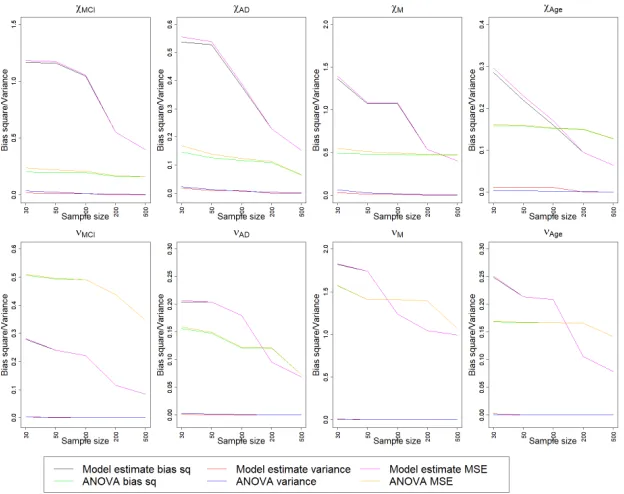
For ANCOVA estimation, we use the weighted least squares technique for the normal model and the generalized linear regression for Poisson regression model for the Poisson link function. We provide table for squared bias and variance of the estimates for the slope parameters for largest sample size in a table. We present a comparison plot of squared bias, variance and MSE of the estimates across different sample sizes in Figure 2.3 and Table 2.1.
For misspecified case as well we provide squared bias, variance and MSE of the estimates for the largest sample size 500 in Table 2.2. There is also a comparison plot of bias square, variance and MSE of estimates across different sample sizes in Figure 2.5.
Table 2.1: Comparison of estimation accuracy forn= 500 in well-specified case
Bayes
ANCOVA
Square bias
Variance
MSE
Square bias
Variance
MSE
χ
MCI0.01
0.0001
0.0101
0.02
0.0015
0.0215
χ
AD0.00
0.0001
0.0001
0.02
0.0013
0.0213
χ
M0.00
0.0001
0.0001
0.00
0.0012
0.0015
χ
Age0.01
0.0000
0.0100
0.03
0.0002
0.0302
ν
MCI0.00
0.0000
0.0000
0.01
0.0003
0.0103
ν
AD0.01
0.0000
0.0100
0.03
0.0002
0.0302
ν
M0.00
0.0000
0.0000
0.00
0.0002
0.0012
ν
Age0.01
0.0000
0.0100
0.02
0.0000
0.0200
Figure 2.3: Plot of squared bias and variance for different parameters against sample sizes for Bayesian method and ANCOVA estimates in the well-specified case.
for all the cases. From Figure 2.3 we conclude that proposed Bayesian method performs better than ANCOVA after sample size 25. In Figure 2.4, for misspecified case we observe both of the Bayesian and ANCOVA estimates are in similar color range with the truth for most of the cases. So, both of the methods could estimate the fixed effect for most of the parameters. In Figure 2.5 we can compare the two estimates quantitatively. The two methods show comparable performance as sample size increases for all of the eight parameters.
2.5
Real data analysis
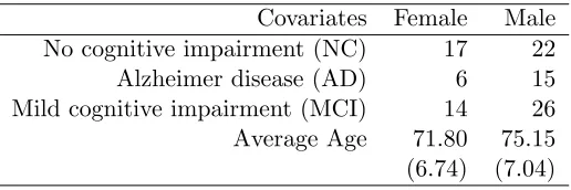
We analyze a real dataset with 100 individuals, collected from ADNI. A demographic summary of the data is provided in Table 2.3. The baseline subject is a female subject of average age with no cognitive impairment. The plot of the estimates, obtained from the proposed Bayesian method are given in Figure 6.
Figure 2.5: Plot of squared bias and variance for different parameters against sample sizes for Bayesian method and ANCOVA estimates in the misspecified case.
similar to the one used in White and Ghosal (2014). We fit a Gaussian mixture model (GMM) for the marginal density ofAi,j, Ψ(a) =Pki=1ωkφ(a, µk, σk). We choose the value ofkbetween
3 to 5 depending on the AIC value after fitting the model. The R package mixtools is used for estimation of GMM. Then based on the highest posterior probability component i.e. the l for whichωl is maximum in the mixing vectorω, we find the significant edges and that highest
posterior probability component µl is the representative value for the estimated matrix. The
posterior probability for each edge Aij is defined by the fraction ωlφ(AΨ(Aijij,µ)l,σl). The number of
significant edges is obtained based on 5% tolerance level of the posterior probabilities of different edges i.e. the fraction from the previous line. There are total 3486 many edges including self edges.
Most significant 50 edges are plotted for each parameter of interest. The edge-widths are proportional to the level of significance, more width means more significant. The colored circles are the different regions and their names are mentioned in the legend. These plots are in 2.6, 2.7 and 2.8.
Table 2.2: Comparison of estimation accuracy forn= 500 in misspecified case
Bayes ANCOVA
Square bias Variance MSE Square bias Variance MSE
χMCI 0.40 0.0080 0.3988 0.19 0.0020 0.1608
χAD 0.15 0.0070 0.1524 0.06 0.0011 0.0657
χM 0.40 0.0001 0.4018 0.46 0.0024 0.4714
χAge 0.06 0.0005 0.0635 0.12 0.0002 0.1269
νMCI 0.08 0.0003 0.0842 0.49 0.0002 0.3469
νAD 0.07 0.0002 0.0691 0.07 0.0002 0.0733
νM 0.99 0.0004 0.9953 1.07 0.0002 1.0710
νAge 0.07 0.0001 0.0786 0.14 0.0000 0.1416
Table 2.3: Demographic table
Covariates Female Male No cognitive impairment (NC) 17 22 Alzheimer disease (AD) 6 15 Mild cognitive impairment (MCI) 14 26 Average Age 71.80 75.15 (6.74) (7.04)
between two different regions. The significant edges for these two plots are similar. Both of the two are related to the presence or absence of edges or number of edges. Most significant edges for covariates related to disease states involve edges related to memory management regions banks of the superior temporal sulcus, entorhinal, and transversetemporal. In the network plots for covariate ‘Age’ there are above mentioned regions along with edges related to cuneus. It also involves medial orbito frontal. For the covariate ‘Gender’ most of the significant edges are related to the regions responsible for memory management and visual processing.
2.6
Large-sample Properties
We consider an abstract setting a fixed J number of nodes, which need not be specifically restricted to the problem of connectome. The observations follow the data generating process in (2.1) and parameters are given by (2.2). Instead of being specific about predictors like in 2.3, we consider that there are a fixed numberdof covariates denoted by Zi = (Zi1,· · · , Zid)0,
i = (1,· · ·, n), where n is the sample size. The asymptotics is in terms of n → ∞. Then regression coefficients χjk, βjk, νjk ared-dimensional. For notational convenience, we write=
Figure 2.7: Effect of covariates on connection-probability, each circle denotes different cortical brain regions and edge-widths are proportional to the degree of significance of that edge.
consider for each pair (i, :i= 1, . . . , n; = 1, . . . J2) that there are p dimensional covariates Xi such that Xi = (1, Zi0)⊗e, where e is vector of length J2
with one at th position and ⊗stands for the Kronecker product. Posterior consistency is established in Kim and Kim (2011) for mixed effect model with binary data P(Yij = 1|Xij, Zij) = H(X
0
ijβ+Z
0
ijbi) where
β = (β1, . . . , βp)0 and Xij = (Xij1, . . . , Xijp)0 are p-dimensional vectors standing respectively
for fixed effects and the corresponding regressors, b= (b1, . . . , bq)0 and Zij = (Zij1, . . . , Xijq)0
areq-dimensional vectors standing respectively for random effects covariates with distribution functionF and the corresponding regressors. LetH be a known increasing and symmetric link function. Then we can rewrite our model as
logWi=Xi0 χ
∗+η
1i+i, i∼N(0, σ2/Ni),
Ξi ∼Bin(1, H(Xi0 β
∗
+η2i)),
Ni|{Ξi= 1} ∼Poisson(eλi), λi =Xi0ν
∗
+η3i,
η1i ind
∼ F1, η2i ind
∼ F2, η3i ind
∼ F3, i= 1, . . . , n;
is denoted byθ= (χ∗, β∗, ν∗, F1, F2, F3). Note that in our setup q= 1 and Zi10 = 1 for all i.
We proceed like the posterior consistency result of Kim and Kim (2011) with appropriate modifications, and show that the arguments extend to cover the normal and Poisson regression mixed effect regression models as well. More specifically, their posterior consistency result is established by verifying that the true parameter lies in the Kullback-Leibler support of the prior and constructing uniformly exponentially consistent tests for testing the true point null against a complement of an arbitrary sized neighborhood of the truth and applying the general theory of posterior consistency; see Ghosal and van der Vaart (2017) for details on the gen-eral theory. Using standard arguments, we establish the prior positivity condition for each of the three — binary regression, Poisson regression and normal regression model. To construct the required tests, we proceed like Kim and Kim (2011) who considered mixed effects binary regression models and constructed tests using the arguments given in Amewou-Atisso et al. (2003). However they assumed that the whole real line is the support for the first continuous covariate, which is inconvenient for our application. Under symmetry of the link functionH, we construct the required test without this assumption. We then show that for the normal mixed effect regression model part, the required test is automatically obtained from that in the binary part by viewing binary observations as arising from data-coarsening of normal observations. For the Poisson regression part, we construct the required tests directly using ideas used for the binary regression model.
Let the parameter space forF1,F2 andF3 be denoted byF1,F2 and F3 respectively. Thus
the parameter space for θ is Rp×Rp×Rp× F1× F2× F3. We consider a prior ˜Γ1 for F1, ˜Γ2
for F2 and ˜Γ3 for F3 independently, and independent of F1, F2 and F3, we consider priorsα1
forχ∗,α2 forβ∗ and α3 forν∗ respectively. Let χ0,β0 and ν0 be the true values of χ∗,β∗ and
ν∗ respectively and F10, F20 and F30 be the true random effects distributions of η1, η2 and η3
respectively. Call (χ0, β0, ν0, F10, F20, F30) to beθ0. We make the following assumptions.
Notation: A set Qn is (asymptotically) non-null if lim inf |Qnn| >0, where |.| denotes
cardi-nality of a set.
• (RE). Random effect distribution: The random effectsη1i, η2i andη3i have mean zero and
symmetric symmetric distribution.
• (SG). Subgaussian tail: The true distribution F0
1 has subgaussian tail:F10(z:|z|> t) .
exp(−bt2) for some constant b >0.
• (Supp). Support of the prior: The true distributions Fi0 ∈ supp(Γi), i = 1,2,3, and
χ0 ∈ supp(α1), β0 ∈ supp(α2) and ν0 ∈supp(α3), where supp stands for the topological
• (CA1) For all , k, there exists an 0 such that {i: Xik > 0} and {i:Xik <−0} are
non-null.
• (CA2) Consider, for anyk, Pn,k, ={i: 1≤i≤n, Xik> 0},
Pn,k,0 ={i: 1≤i≤n, Xik<−0},
An,k, ={i: 1≤i≤n, Xik,0 −β−0≤0}.
We assumeAn,k,∩Pn,k,0 ,An,k,c ∩Pn,k,,Acn,k,∩P
0
n,k, andAn,k,∩Pn,k, are all non-null.
CA2 is sufficient. For our model if CA2 holds for a fixed , then CA1 and CA2 only for that are together sufficient.
• The link functionH is symmetric and increasing.
Theorem 2.1. Under the assumed conditions, the posterior for θ is consistent at θ0.
The first assumption (RE) is very standard assumption for random effect when there is a intercept term in the model. The assumption of symmetry is crucial since we drop the as-sumption that the whole real line is the support of the first continuous covariate made in Kim and Kim (2011). A prior that complies with the symmetry restriction is a random scale mixture of normal prior. For this prior, F is represented as F = R
φσ(·)dG(σ) and the
mix-ing distribution G is given a prior distribution with large weak support. In particular, if G is given a Dirichlet process prior, the resulting prior is a Dirichlet process scale mixture of normal (DPSMN) prior. We used this prior in our methodology, but for posterior consistency we allow much more general priors. Our only requirements are that the true distribution of the random effects belongs to the weak support of the prior and has finite mean. The random scale mixture a prior generates symmetric strongly unimodal densities, and hence in order to meet the support requirement, the corresponding true distributionF0 must also be of the form
of a scale mixture of normal F0 =
R
φσdG. Then the conditions hold if G0 is contained in
much weaker condition R
log(1 + σ)dG∗(σ) < ∞; see Ghosal and van der Vaart (2017) for the details. The condition of finite mean can be ensured easily. For the DPSNM prior, writing F =R
φσ(.)dG(σ) andG∼DP(M, G0), finiteness of the mean ofF is ensured with probability
one ifR
σdG0(σ)<∞, then this will imply
R
σdG(σ)<∞. Since G∼DP(M, G0), G0 =EG.
Since G0 = N(0,1), above conditions hold. However as we put DPSMN prior, much weaker
condition R
log(1 +σ)dG0(σ)<∞ is sufficient. The condition (Supp) that the true parameter
values are in the supports of the corresponding prior distributions is a basic requirement for posterior consistency. The subgaussianity condition (SG) on the true distributions of random effects allows transition from weak support to Kullback-Leibler support, which is again vital for posterior consistency; see Chapter 6 of Ghosal and van der Vaart (2017).
In the methodology we actually used a graphon function to reduce dimension of the re-gression coefficients for each pair of regions. Clearly, then the prior is concentrated on a lower dimensional space, and hence to satisfy the support requirements, the truth must have a similar graphon based structure. Once the support condition is ensured, posterior consistency of the resulting Bayesian procedure can be derived as a corollary from Theorem 2.1. For our model
χ= (((µ0)),((χMCI)),((χAD)),((χM)),((χAge))),
β = (((π0)),((βMCI)),((βAD)),((βM)),((βAge))),
ν = (((λ0)),((νMCI)),((νAD)),((νM)),((νAge))).
The parameter for each pair follows the graphon structure in (2.4) in reduced parameter space. In the abstract setting we can describe this as
χ=ζ(µ0, χMCI, χAD, χM, χAge, ξ, δ),
β=ζ(π0, βMCI, βAD, βM, βAge, ξ, δ),
ν=ζ(λ0, νMCI, νAD, νM, νAge, ξ, δ),
where the function ζ is continuous is its arguments and matrices are replaced by the corre-sponding graphon functions. Let the parameter space for graphon functions be L = class of real-valued smooth continuous functions on [0,1]2. After this reparametrisation the new param-eter will be ˜θ = (µ0, χMCI, χAD, χM, χAge, π0, βMCI, βAD, βM, βAge, λ0, νMCI, νAD, νM, νAge, ξ, δ).
The parameter space of ˜θisL15×[0,1]2. Let ˜θ
0 be the null value of ˜θ. All the prior assumptions
will continue to hold except for the support condition of the prior of the fixed effects (Supp.). New support condition is
true graphon functions.
Corollary 2.2. Under the support assumption of prior ofθ with (Supp) assuption replaced by (RSupp), the posterior for θ˜is consistent at θ˜0.
2.6.1 Proof
We use the consistency result, given in theorem 2 of Amewou-Atisso et al. (2003). To proceed with this consistency result, we show prior positivity of the parameters and construct exponen-tially consistent tests. The whole likelihood can be split into three parts for the three model. It suffices to show prior positivity for the three models separately (i) normal, (ii) binomial and (iii) Poisson model.
Lemma 2.3. Consider a kernel function K(x;υ, η), which is continuous in υ and η. For a fixed parameter υ0 and distribution F0 of η if for a sequence (υn, Fn) such that Fn F0 and
supη∈RkK(x;υn, η)−K(x;υ0, η)k 0, then we have
R
K(x;υn, η)dFn(η)
R
K(x;υ0, η)dF0(η). (Here denotes convergence.)
Proof. We can show k
Z
K(x;υn, η)dFn(η)−
Z
K(x;υ0, η)dF0(η)k ≤
Z
kK(x;υn, η)− K(x;υ0, η)kdFn(η) +
Z
K(x;υ0, η)k(dFn(η)−dF0(η))k.
This inequality proves the statement in the lemma. Prior positivity
(i) Normal model
Let Wi∗ = (logWi1, . . . ,logWi)0, Ni = (Ni1, . . . , Nip)0, Xi = (Xi1, . . . , Xip)0 and Di =
P
Ni. Then we can write
pi,θ(Wi∗|xi) =
Z R Y 1 √
2πσ/pNi
φ
logWi−Xiχ−η1i
σ/p Ni
dF1(η1i).
Defining ¯σ = maxσ/
p
Ni andσ = minσ/
p
Ni and vi =Pk|Xik|, we obtain
pi,θ(Wi∗|xi)≥
Z R Y 1 √
2πσ¯φ
logWi)−Xiχ−η1i
σ
dF1(η1i)
≥ Z B1
−B1
1 2√2πσ¯φ
|P
log(Wi)|+M2Pvi+B1
σ
Let Ti =|PlogWi|. For some positive constant cdepending on B1, we have that
pi,θ0(W
∗
i|xi)/pi,θ(Wi∗|xi).exp(cTi2). This implies that for someδ0 >0,
EF0 1
pi,θ0(W
∗
i|xi)
pi,θ(Wi∗|xi)
δ0
<∞. (2.6)
For two probability densities f and g, define the Hellinger distance dH by d2H(f, g) =
R
(√f−√g)2, the Kullback-Leibler divergenceK(f, g) =R
flog(f /g) and the Kullback-Leibler variation V(f, g) =R flog2(f /g). Applying Theorem 5 of Wong and Shen (1995), from (2.6), we obtain
K(pi,θ(Wi∗|xi), pi,θ0(W
∗
i|xi)).21log
1 1
, V(pi,θ(Wi∗|xi), pi,θ0(W
∗
i|xi)).21log2(1/1),
whenever 1 =dH(pi,θ(Wi∗|xi), pi,θ0(W
∗
i|xi))<1/2. Thus to verify the condition on
Kullback-Leibler support, we only need to verify that Hellinger neighborhoods of pi,θ0(W
∗
i |xi) have
pos-itive prior probabilities, or equivalently L1-neighborhoods since the Hellinger distance induces
the same neighborhood system as theL1-distance on probability densities. In view of Lemma 2.3,
the condition is ensured by the assumed support condition (Supp). (ii) Binomial model
Prior positivity follows from the argument in Kim and Kim (2011). They showed that if β converges toβ0 andF2 converges weakly toF20, then Kullback-Leibler divergence and variation
(write these explicily) tend to zero. (iii) Poisson model
We can write the probability mass function of the observationNi as
pi,θ(Ni|xi) =C
Z
R
Y
(exp −eη3ieXi0ν eη3ieXi0νNi)dF
3(η3i)
=C Z
R
exp −eη3iX
eXi0ν+η
3i X Nij ×Y j
(eXi0ν)NidF
3(η3i), (2.7)
whereC−1 =Q
Ni! is free of the parameters.
By applying Jensen’s inequality and then using the obvious fact that Ni for any is less
than or equal to its sum over the argument, we can write Q
(e
Xi0ν)Ni as
(exp( P
NiXi0ν
P
N i
))Ni ≤
P
NijeX
0
iν
P
Ni
PNi
≤ X
eXi0ν
P
Ni
Substituting above inequality in (6) and observing that the integrand is maximized atη3i=
log(P
jNi/
P
e X0
iν), we obtain the upper bound for (2.7) as
pi,θ(Ni|xi)≤C(
X
j
Nij)
P
jNijexp(−X
j
Nij) =CDiDie
−Di,
whereDi=PNi.
Letting vi=|Xi|and max|ν|=M3, it follows that pi,θ(Ni|xi) is lower bounded by
C 2
Z B3
−B3
exp −eη3iX
eviM3+η
3i X Ni X
e−viM3PNi
dF3(η3i),
= C 2 exp
−eB3X
eviM3 + (B
3+ log(
X
e−viM3)D
i
,
which leads to the estimate pi,θ0(Ni|xi)/pi,θ(Ni|xi) . D
Di
i . Observe that if N is a random
variable distributed as Poisson with parameterλ >0, then for anyδ <1, E exp(δNlogN)<∞. This holds because logn!≥nlogn−nand thatP∞
n=1exp(δnlogn+nlogλ−nlogn+n)<∞
whenverδ <1. Therefore by Theorem 5 of Wong and Shen (1995), we obtain the bounds K(pi,θ(Ni|xi), pi,θ0(Ni|xi)).
2 2log
1 2
, V(pi,θ(Ni|xi), pi,θ0(Ni|xi)).
2 2 log 1 2 2 ,
where 2 = dH(pi,θ(Ni|xi), pi,θ0(Ni|xi)) < 1/2. By Lemma 2.3 and the assumed condition
(Supp), the condition on the Kullback-Leibler support is verified. Test construction
(iii) Normal model
If we reduce the data into binary observations by defining Si =I(Wi0 ≥0). Then Si will
follow a probit model. If we can construct tests for this reduced data, test construction for the whole data will continue to hold. Test construction for binary data is given below for a symmetric increasing link function. This construction will hold for probit model as well.
(iii) Binomial model
Tests for the binary data with symmetric increasing link function are constructed below.
Let,
T1l(∆1,∆l) ={(β∗, F2) :|β1∗−β01| ≤∆1,|βl∗−βl0|>∆l},l= 2, . . . , p
T1p+1(∆1, . . . ,∆p+1) ={(β∗, F2) :|β1∗−β10| ≤∆1, l= 1, . . . , p anddw(F2, F20)>∆p+1}.
Consider, g(x) =EF2[H(x+η2i)]−EF0
2[H(x+η2i)].
Kn={i: 1≤i≤n, g(Xi1,0 −1β−01+Xi11β10)≤0},
Pn={i: 1≤i≤n, Xi11≥0},
An={i: 1≤i≤n, Xi1,0 −1β−01≤0}.
Notation: A set Qn is (asymptotically) non-null if lim inf |Qnn| >0, where |.| denotes
cardi-nality of a set.
We have g(∞) =g(−∞) = 0 and g(x) =−g(−x) because H(x) +H(−x) = 1. This implies g(0) = 0. We have H00(x) = −H00(−x), this follows g00(x) = −g00(−x). We have g00(0) = 0, so x= 0 is a point of inflection. If F2 6≡F20, we would find an interval [−a, a] such that g(x)6= 0
for x ∈ [−a,0). There are two possibilities g(x) and x are of same sign or of opposite signs. Both of the two cases are equivalent. Let at x=±t,g0(x) = 0. We show test construction for the case where g(x) and x are of same sign. So, we have g(x) >0 for x ∈(0, a] and g(x) <0 forx∈[−a,0). We have,EF2,β(Ii1)−EF20,β0(Ii1) =EF2H(X
0
i1β+η2i)−EF2H(X
0
i1β0+η2i) +
g(Xi10 β0). We can create difference in mean if either Xi10 β ≤ Xi10 β0, Xi1,0 −1β−01 +Xi11β10 ≤ 0
or Xi10 β > Xi10 β0, X0
i1,−1β−01+Xi11β01 > 0. To summarize difference in mean will exists when
(Xi1,0 −1β−1 −Xi1,0 −1β−01+Xi11(β1−β01))(Xi10 β0) > 0. Assumption CA2 will ensure Kn∩Pn0,
Knc∩Pn,Knc∩Pn0 and Kn∩Pn are non-null.
Forβ1−β10 >∆1, (Xi1,0 −1β−1−Xi1,0 −1β−01+Xi11(β1−β10))(Xi10 β0)>(Xi1,0 −1β−1−Xi1,0 −1β−01+
Xi11∆1)(Xi10 β0), whenXi11(Xi10 β0) is positive which is true asKn∩PncandKnc∩Pnare non-null.
Above inequality will be greater than zero for the case Xi1,0 −1β−1 > Xi1,0 −1β−01 with elements
from Knc ∩Pn and for Xi1,0 −1β−1 < Xi1,0 −1β−01 we choose elements from Kn∩Pnc. The other
possibility isβ1−β10<−∆1. Then we have, (Xi1,0 −1β−1−Xi1,0 −1β−01+Xi11(β1−β10))(Xi10 β0)>
(Xi1,0 −1β−1−Xi1,0 −1β0−1−Xi11∆1)(Xi10 β0) with elements fromKn∩Pnand Knc∩Pnc. This time
we chooseKnc∩Pnc forXi1,0 −1β−1 > Xi1,0 −1β−01 case and Kn∩Pn forXi1,0 −1β−1< Xi1,0 −1β0−1.
For T1l, the difference in mean is created when