ABSTRACT
FERNANDO, PAUL R. Adding scalability to IBIS using AMS languages. (Under the
direction of Dr. Paul Franzon.)
From 1993 to about 1998, IBIS remained THE digital IO buffer model format. But as
the operating frequencies & complexity of I/O buffers increased, IBIS has been left behind in
favor of SPICE models, since IBIS is inaccurate or unable to model these advanced buffers.
This trend brings the industry back toward a single EDA vendor solution, which is what IBIS
was designed to prevent. In an effort to relinquish these shortcomings, multi-lingual model
extensions were added to IBIS Version 4.1. Specifically: Berkeley-SPICE, VHDL-AMS and
Verilog-AMS files.
These extensions in IBIS 4.1 give IBIS practically unlimited behavioral and structural
modeling capabilities as well as more accuracy. The problem is that the AMS languages have
been slow in making their way into SI tools and the SI community; mainly due to the
associated learning curve, since AMS is relatively new to the SI world.
The solution was to build an AMS library of tool independent basic elements
(“element library”) and a separate “template library” which would contain the models of
complex buffers (Pre-emphasis, LVDS, DDR2 etc). The templates would be created by
instancing elements from the “element library”. An IBIS to AMS converter would convert
conventional IBIS files into AMS format and provide the data for the template. The IBIS
macro-modeling committee was created in July 2005 with these main goals in mind.
This thesis deals with the new AMS macro-modeling methodology put forth by the
IBIS macro-modeling committee and the contributions I made to it as its only student
member. My specific contribution was the IBIS to AMS (ibis2ams) converter tool. The thesis
also presents the updates I made to the IBIS plotting utility (s2iplt) and the spice to IBIS
Adding scalability to IBIS using AMS languages
by
Paul R. Fernando
A thesis submitted to the Graduate Faculty of North Carolina State University
In partial fulfillment of the Requirements for the degree of
Master of Science In
Computer Engineering
Raleigh, NC
2006
Approved by:
________________________
Dr. Paul Franzon
Chair of Advisory Committee
________________________ ________________________
DEDICATION
To my Parents, Teachers,
iii
BIOGRAPHY
Paul Fernando was born in Colombo, Sri Lanka, in October 1982. He joined
Louisiana State University in Baton Rouge, LA at age 16 and graduated cum laude in May
2003 majoring BS in Computer Engineering with minors in Mathematics and Computer
Science. He received his second BS in Electrical Engineering in December 2003. He interned
at Dallas Semiconductors (Maxim Integrated Products) in Dallas, TX in the summer of 2002
where he was introduced to IBIS modeling and NCSU’s s2ibis toolkit for the first time.
He began his MS in Computer Engineering at North Carolina State University in Fall
2004 under the supervision of Dr. Paul Franzon. A Summer and Fall co-op in 2005 at Analog
Devices, Boston MA, focused, among many other things, on creating a novel flow for fast
and accurate IBIS model generation within the company. After working with state of the art
IO buffer models at ADI, it became clear that IBIS required major additions to retain
accuracy. Since then, he has being working with the IBIS macro-modeling committee
consisting of IBIS industry leaders from Intel, Cisco, Cadence, Mentor Graphics, Teraspeed
Consulting, SiSoft etc. to develop a new methodology which incorporates AMS languages to
IBIS.
He will begin work in May 2006 as a full time employee in the Visual Signal
ACKNOWLEDGMENTS
A warm “Thank You” to Dr. Paul Franzon for the support and guidance he provided
me throughout my Masters program. His help was imperative in gaining my co-op at Analog
Devices last year which resulted in me getting my full-time offer even before I finished the
co-op. I’d also like to acknowledge the members of my committee, Dr. Rhett Davis and Dr.
Kevin Gard. Together with Dr. Maysam Ghovanloo they, among many other things, made
my first semester at NCSU a very challenging, exciting and fulfilling one. Ambrish Varma
played a vital role during my MS program right from the start. The valuable discussions we
had proved to be essential for my thesis.
Thank you, Dr. Bob Evans, for putting me in touch with Mike LaBonte and the IBIS
macro-modeling committee. And also for teaching, what is arguably, one of the best Signal
Integrity classes on the planet.
I would like to express my gratitude to the entire IBIS macro-modeling committee.
Specifically, Arpad Muranyi (Intel), Mike LaBonte (Cisco), Todd Westerhoff (Cisco), Walter
Katz (SiSoft), Barry Katz (SiSoft), Ken Willis (Cadence), Ian Dodd (Mentor), Sam Chitwood
(Sigrity), Bob Ross (Teraspeed) & Scott McMorrow (Teraspeed).
My thanks go out especially to Arpad & Mike. Your help added an industrial
dimension to my work. Thanks Arpad, for the extensive feedback while developing ibis2ams.
At the time this thesis was authored, NCSU had no simulator capable of handling
AMS languages. Dolphin Integration provided a free license for SMASH, its mixed signal
(AMS) simulator worth $25k. Thank you to Gilles Depeyrot & Thierry Depeyrot of Dolphin
v
TABLE OF CONTENTS
List of Tables . . . vii
List of Figures . . . viii
1. Introduction . . . 1
1.1 Why IBIS? . . . 1
1.2 What is IBIS (I/O Buffer Information Specification) . . . 4
1.3 3-state Driver IBIS data extraction . . . 7
1.4 NCSU’s involvement with IBIS . . . 11
1.5 IBIS Limitations . . . 12
1.6 Thesis Organization . . . 14
2. The AMS Macro-modeling Concept . . . 15
2.1 Introduction . . . 15
2.2 The IBIS Macro Modeling Committee (IBIS-macro) . . . 19
2.3 The IBIS-AMS Macro-model Hierarchy . . . 21
2.4 The simulation algorithm . . . 22
3. The IBIS-to-AMS converter . . . 26
3.1 Introduction . . . 26
3.2 The IBIS-to-AMS Flow . . . 27
4. Results . . . 32
4.1 Introduction . . . 32
4.2 Case study I: Output Buffer . . . 33
4.3 Case study II: Pre-emphasis Buffer . . . 36
4.4 Case study III: Equalized Receiver . . . 42
5. Conclusions & Future Research . . . 45
5.1 Conclusions . . . 45
5.2 Future Research . . . 46
Appendix A: IBIS Macro Library Elements . . . 50
Appendix B: IBIS to Verilog-A converter script . . . 52
Appendix C: The Verilog-AMS “IBIS_IO” model description . . . 73
Appendix D: Simulating the “IBIS_IO” model in Dolphin Smash . . . 86
Appendix E: Case Study I: Output Buffer simulation files . . . 88
Appendix F: Case Study II: Pre-emphasis Buffer simulation files . . . 90
Appendix G: Case Study III: Equalized Receiver simulation files . . . 94
Appendix H: IBIS plotting utility (s2iplt) . . . 97
vii
LIST OF TABLES
Table A.1: Basic Elements . . . 50
Table A.2: Sources . . . 50
Table A.3: Operators . . . 51
Table A.4: Active Devices . . . 51
LIST OF FIGURES
Figure 1.1: Moore’s Law . . . 2
Figure 1.2: 3-state buffer structure . . . 7
Figure 1.3: PU & PD curves . . . 8
Figure 1.4: PC & GC Curves . . . . . . . 9
Figure 2.1: Current IBIS timeline . . . 15
Figure 2.2: Proposed IBIS timeline . . . 16
Figure 2.3: AMS Hierarchy . . . 21
Figure 2.4: IBIS Simulation Circuit . . . 23
Figure 3.1: Simulation Process Diagram . . . 26
Figure 3.2: ibis2ams Convert Manu . . . 27
Figure 3.3: ibis2ams Select IBIS file Dialog . . . 27
Figure 3.4: ibis2ams Select model to convert . . . 28
Figure 3.5: ibis2ams Select process corner . . . 29
Figure 3.6: ibis2ams Select output file name . . . 29
Figure 3.7: Sample Verilog-AMS output file . . . 30
Figure 3.8: Sample VHDL-AMS output file . . . 31
Figure 4.1 Conversion Flow . . . 33
Figure 4.2 Test Circuit . . . 33
Figure 4.3 SMASH GUI . . . 34
Figure 4.4 Output Comparison . . . 35
Figure 4.5 Pre-emphasis Buffer Schematic . . . 37
ix
Figure 4.7 Pre-emphasis Buffer VHDL-AMS code (Part 2) . . . 39
Figure 4.8 Pre-emphasis Buffer Test Circuit . . . 40
Figure 4.9: Pre-emphasis Buffer SMASH GUI . . . 40
Figure 4.10: Pre-emphasis Buffer SMASH Output . . . 41
Figure 4.11: Receiver Schematic . . . 42
Figure 4.12: Receiver VHDL-AMS code . . . 43
Figure 4.13: Receiver SMASH Output . . . 44
Figure D.1: SMASH GUI . . . 86
Figure D.2: SMASH output for Risetime = 0.1ns . . . . . . 87
Figure D.3: SMASH output for Risetime = 0.5ns . . . 87
Figure H.1: s2iplt GUI main interface . . . 98
Figure H.2: s2iplt in50v Power Clamp Curve . . . . . 99
Figure H.3: s2iplt sample PostScript file . . . 100
1. Introduction
1.1 Why IBIS?
The fastest entity in the universe is an electromagnetic (EM) wave traveling in a
vacuum. This velocity is defined as C (3.0*108 m/s). Typically, signals on a PCB travel about
half C. Thus, it takes about 100ps for light to travel from your nose to your eyes [1]. In the
latest electronic systems a signal skew of a few 100ps would be sufficient to corrupt the
information it carries. Given that C is a universal constant it’s easy to see that modern
electronics is reaching a ceiling in terms of signaling speed. Adding to the complexity is that
at high frequencies, conductors no longer act as simple wires. They begin to act as
transmission lines exhibiting high-frequency effects. And as frequencies increase, so do these
complex effects. Transmission line conditions occur when the physical size of a circuit
reaches the wavelength of the highest frequency of interest in a signal. For digital systems,
higher digital frequencies require sharp edge rates which contain high frequency components
(harmonics). Thus, modern board simulations require TL analysis. Nowadays, even clock
trees within a single chip require this analysis. Simulating for these high frequency effects
involves the use of complex 3-D field solvers. If these effects are unaccounted for in high
speed circuit design, the results will almost certainly be disastrous. For this reason,
simulation takes a massive role in validating modern designs as timing gets increasingly
constrained. It is said that all simulations are inaccurate, but some simulations are useful. The
goal in simulation is to obtain the greatest accuracy; the tradeoffs being time, manpower and
[3]
Figure 1.1: Moore’s Law
When the integrated circuit was invented by Jack Kilby in 1958, circuit design split
into two disciplines: Discrete (board-level) and IC (chip-level). Historically, chip level circuit
design has targeted performance (see Fig 1.1), while board level circuit design has targeted
cost. The result has been that while signaling speeds within a microchip have been increasing
exponentially with respect to time, this has not been the case at the board level (chip to chip).
Thus, a majority of the speed bottleneck in modern systems is at the board level. For
example, since the signaling between a CPU and the RAM (bus speed) is too slow, it has
become mandatory to use on-chip memory (Cache) running at the CPU’s core frequency.
Modern processors have more than 4Mb of cache and, based on current trends, increases are
expected. This is also one of the reasons for the recent multi-core trend in CPUs. Even
though these developments take a massive overhead they have been necessary due to the
board level speed bottleneck.
Another distinguishing factor here is that IC level design is (usually) completed
within a single company, while board level design involves components manufactured by a
variety of companies. For example, ASUS designs a motherboard using an Intel CPU,
Micron DRAM, Nvidia GPU etc. For optimum system performance ASUS would require
complete design information about each component before working on its (system level)
design. While sharing design information with a company is complex in itself, sharing this
information between companies would be disastrous to the supplier company’s business. The
netlist would contain process information giving details about the latest FABs & processes
not to mention complete design information. For these (and many more) reasons, companies
would rather not disclose such proprietary information. Thus, the industry standard circuit
simulator, Spice, does not fulfill board-level simulation requirements, since it provides a
complete description of the design as well as process information. Another factor was that
Spice is component centric, and therefore, simulation of massive circuits takes a long time. In
the early 1990s it became clear that a new modeling technique was in order. The technique
4
1.2 What is IBIS (I/O Buffer Information Specification)
IBIS was developed by Intel® Corporation in the early 1990s. IBIS version 1.0 was
issued in June 1993 along with the creation of the IBIS Open Forum. The IBIS Open Forum
comprises of EDA vendors, computer manufacturers, semiconductor vendors, universities,
and end-users. It proposes updates and reviews, revises standards, and organizes summits
related to IBIS. It promotes IBIS models and provides useful documentation and tools on the
IBIS website. In 1995, the IBIS Open Forum teamed up with the Electronic Industries
Alliance (EIA). The main facets of IBIS are that [2]:
1. It protects proprietary information. (No circuit information or process parameters are
disclosed)
2. Non-linear aspects of I/O are modeled as well as package parasitics and ESD structure.
3. It is much faster (upto 25x) than other transistor level simulators such as SPICE.
4. The IBIS model can be provided before silicon. (Pre tape-out)
5. Supported by most SI industry tools.
Given these advantages, IBIS has become the standard for board level Signal
Integrity (SI) simulations.
An IBIS model consists of tabular data made up of current and voltage values at the
output and input pins, as well as the voltage and time relationship at the output pins under
rising or falling switching conditions (with varying output load conditions). This tabulated
data represents the ‘behavior’ (including non-linear characteristics) of the buffer. IBIS only
deals with digital buffers & signals.
An IBIS model is (primarily) used by an SI tool to calculate fundamental signal
Potential problems that can be analyzed by means of these simulations include the degree of
energy reflected back to the driver from the wave that reaches the receiver due to
mismatched impedance in the line; crosstalk; ground and power bounce; overshoot;
undershoot; and line termination analysis, among others [4].
IBIS is an accurate model since it takes into account nonlinear aspects of the I/O
structures, the ESD structures, and the package parasitics. It has several advantages over
other traditional models such as SPICE. Thus, for example, the simulation time can be up to
25 times less, and IBIS does not have the non-convergence problem SPICE does. In addition,
IBIS can be run on any industry-standard tool since most Electronic Design Automation
(EDA) vendors support the IBIS specification.
IBIS files can be generated using bench measurements or by running (SPICE)
simulations. The second method is more frequently used since it takes the least amount of
overhead from the model maker’s perspective. A second reason is that the bench results are
directly impacted by the accuracy of the measurement equipment used as well as other
environmental effects. A third reason is that IBIS files created from simulations can be
provided to customers before tape-out. Therefore, customers get a head start on system level
design before first silicon.
IBIS models are characterized under three corner conditions. The “slow” corner is
characterized under minimum supply voltage, maximum temperature and slow process
parameters (device models). The “fast” corner is characterized under maximum supply
voltage, minimum temperature and fast process parameters (device models). The “typical”
6
The IBIS specification supports many kinds of drivers: Input, Output, I/O, 3-state,
Open_drain, I/O_open_drain, Open_sink, I/O_open_sink, Open_source, I/O_open_source,
Input_ECL, Output_ECL, I/O_ECL, 3-state_ECL, etc [6]. IBIS does not support analog
buffers.
In the next section, a 3-state driver will be used as an example to explain what
1.3 3-state Driver IBIS data extraction
[2]
Figure 1.2: 3-state buffer structure
The basic structure of a 3-state driver is given above.
The PU & PD MOS devices form the 3-state driver: the output is hi when only the PU
PMOS is on; the output is low when only the PD PMOS is on; the output is hi-z when both
MOS devices are off. The package pin will be floating in the final case.
The PC & GC diodes form the ESD (Electro-static discharge) protection mechanism
used to protect the chip from high voltages that may appear on the pad due to external
environmental factors.
C_comp lumps the capacitance of all the devices on the die pad. This capacitance can
be approximated by adding the capacitances of the PU, PD, PC & GC components on the
(on-die) pad node. This value is typically in the single digit Pico Farad range. Unfortunately,
NCSU’s s2ibis utility cannot extract this value.
The [package] RLC values reflect the (lumped) parasitic RLC that is present in the
by the package manufacturer. Alternatively, the [Package Model] keyword may be used to
provide an RLC matrix for more accuracy.
The data captured in an IBIS file consists of the following (Note: package parasitics
& C_comp are not included when running these simulations):
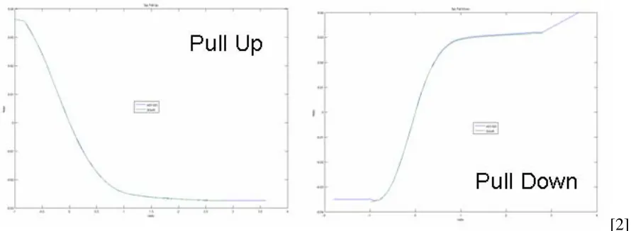
1. Pullup and Pulldown V-I tables
With the output set high, the output node is swept from –Vcc to 2Vcc while the corresponding current through the output node is measured. This V-I table
forms the Pullup curve. For the Pulldown curve, the output is set low and the same measurement is repeated. For the Pullup curve, the voltages must be
made Vcc relative by subtracting the values from Vcc. Finally, the clamp
effects (obtained from the next set of simulations) must be subtracted from
these results to remove the clamping effects.
[2]
Figure 1.3: PU & PD Curves
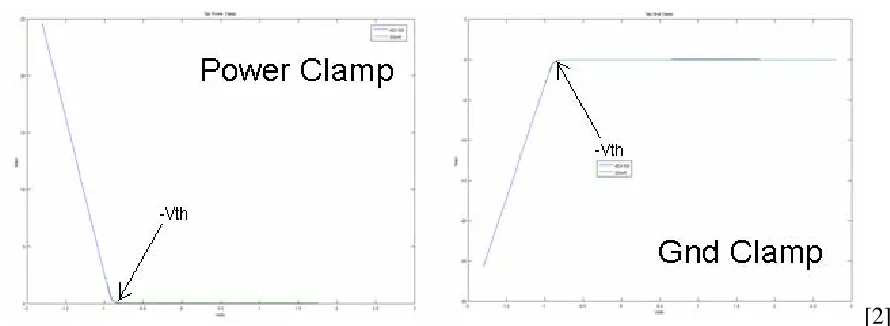
2. Power clamp and Ground clamp V-I tables
The output is set to hi-z for these measurements. The output is swept from
–Vcc to Vcc for the Ground clamp curve, while the output is swept from Vcc
to 2Vcc for the Power clamp curve. As in the Pullup case, the Power clamp
curve must be made Vcc relative by subtracting each the value from Vcc.
[2]
Figure 1.4: PC & GC Curves
3. Ramp rate (dV/dt)
The output is connected to a shunted 50Ohm resistor (standard load). The
output is switched from low to high and high to low and the voltage-time
variation from the 20% voltage point to the 80% voltage point is measured for
each case. This is used to calculate the dV/dt for the rising and falling case
respectively.
4. Rising and Falling V-time tables
The setup is similar to the Ramp rate setup but the resistor value may be
varied. In this case the output voltage is measured with respect to time. The
10
configuration). Thus, at least four of these tables are required (i.e. rising with pulldown resistor, rising with pullup resistor, falling with pulldown resistor &
falling with pullup resistor.) for a complete set of data.
NCSU s2ibis is commonly used to convert buffer spice netlists to IBIS format. It
supports various favors of spice.
1.4 NCSU’s involvement with IBIS
NCSU has been at the forefront of IBIS development since its conception over a
decade ago.
The initial specification for IBIS (version 1.0) was issued in June 1993 with the
formation of the IBIS Open Forum. The industry’s first Spice to IBIS conversion utility,
S2IBIS version 1 was released in July 1994 by the Electronics Research Lab at NCSU. Since
then, NCSU has released S2IBIS2 and S2IBIS3 which met the demands of IBIS
specifications version 2 & 3 respectively.
The current version, S2IBIS3 was written in Java and is capable of handling
non-convergence issues in spice. It is platform independent. It is compatible with the following
spice simulators: Hspice, Pspice, Spice2, Spice3, Spectre & Eldo. It also handles the IBIS
v3.2 specific keywords such as [series MOSFET], [series pin mapping] and [series switch
groups].
In 1995 NCSU introduced the IBIS plotting utility (s2iplt).
S2IBIS has clearly proven to be THE industry standard tool for spice to IBIS
conversion; making NCSU the primary university involved with IBIS.
As part of this thesis, s2iplt (IBIS wave plotting utility) & s2ibis (Spice to IBIS
12
1.5 IBIS Limitations
Since IBIS as a standard began to evolve in the 1990s it has gone through several
updates. IBIS Version 4.1 (Released in February 2004) is the current standard at the time of
this publication. Even thought these updates have added new keywords to improve the
scalability & accuracy of IBIS, the time lag between the emergence of new I/O buffer
technologies, their support in the IBIS specification and support in IBIS simulators has
continued to grow. As the operating frequencies of I/O buffers increase, many model makers
and/or users leave IBIS behind in favor of SPICE models. Since most semiconductor vendors
support their models with a single vendor's version of SPICE, this trend brings the industry
back towards a single EDA vendor solution, which is what IBIS was designed to prevent.
It is quite clear that IBIS is currently having a hard time keeping up with advanced
technology modeling (For example modeling pre/de emphasis buffers, LVDS & DDR2).
However, as mentioned in section 1.2, behavioral modeling has significant advantages over
SPICE.
In version 4.1, multi-lingual model extensions were added to IBIS so that it could
recognize Berkeley-SPICE (Version 3F5), VHDL-AMS (IEEE Std. 1076.1-1999) and
Verilog-AMS (IEEE 1364-2001) files. These files can be specified using the [external
circuit] keyword. These extensions in IBIS 4.1 give IBIS practically unlimited behavioral and
structural modeling capabilities as well as more accuracy. The problem is that the AMS
languages are slow in making their way into SI tools and the SI community. There are many
reasons for this problem [7]:
1. Model developers must learn a new language (*-AMS)
3. Few *-AMS models exist.
However, there is a current need for modeling and simulating advanced buffers.
The purpose of this thesis is to provide an industry standard methodology that helps
14
1.6 Thesis Organization
The remainder of this thesis is organized as follows:
Chapter 2 describes the AMS Macro-modeling concept.
Chapter 3 gives examples and results in the form of case studies.
Chapter 4 provides Conclusions & Future Research.
As part of this thesis, s2iplt (IBIS wave plotting utility) & s2ibis (Spice to IBIS
converter) were updated to feature GUI interfaces & other functions. These are described in
Appendices H & I respectively.
2. The AMS Macro-modeling Concept
2.1 Introduction
[8]
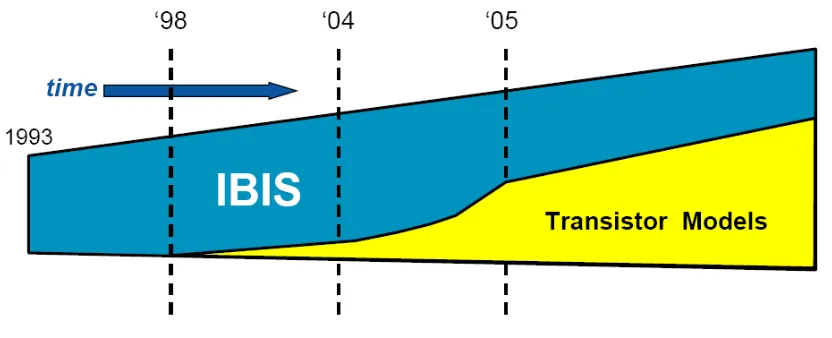
Figure 2.1: Current IBIS timeline
From 1993 to about 1998 IBIS remained THE digital IO buffer model format [8]. But
as operating frequencies continued to increase, IBIS became less accurate in most cases and
outright unusable in others. IBIS is running out of steam, and if nothing is done about this
situation, the industry will end up with nothing but SPICE (transistor) models (figure 4.1).
But clearly, SPICE is not a viable long term solution- mainly due to its long simulation times
& proprietary information [8].
Simply adding new keywords to IBIS will not be a viable solution when it comes to
keeping up with the ever faster evolution of complicated buffers. Clearly the future is in the
adoption of flexible modeling languages, such as the ones accepted by IBIS 4.1. Specifically,
Berkeley-SPICE (Version 3F5), VHDL-AMS (IEEE Std. 1076.1-1999) and Verilog-AMS
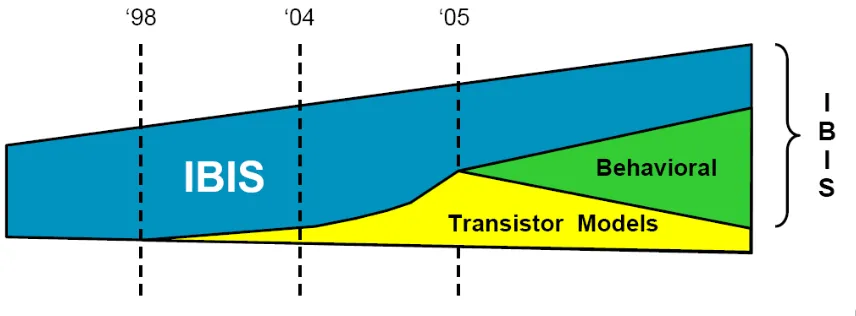
Thus, the evolution of IBIS is expected to encompass behavioral modeling and
continue as shown in (figure 4.2). Simple buffers will continue to be modeled in ‘normal’
IBIS while state of the art high speed buffers (where accuracy is more important) will be
modeled using behavioral languages. It is also possible that IBIS models will be purely
behavioral in the not-too-distant future.
[8]
Figure 2.2: Proposed IBIS timeline
Behavioral modeling offers several benefits:
1. Fast simulation times
2. IP protection
3. Template based (therefore easier and faster to create)
4. Many tools support it (Verilog & VHDL are very popular)
5. Direct link to IC design
The most popular behavioral modeling languages are Verilog & VHDL.
Traditionally, behavioral modeling has only supported the digital domain. This wouldn’t be
sufficient for IBIS since its table’s exhibit analog behavior. Recently, Verilog & VHDL were
enhanced with Analog Mixed Signal (AMS) extensions which added capabilities of modeling
analog & mixed signal behavior. Given these extensions, Verilog-AMS & VHDL-AMS were
chosen to strengthen the IBIS paradigm. For high-speed buffer modeling, *-AMS combines
the behavioral-modeling capability of IBIS with the unrestricted topology description
functionality of Spice [11].
AMS supports a variety of modeling styles - a buffer can be described purely
behaviorally, but also in a structural manner with a circuit netlist and semiconductor process
description. In addition, the netlist portion of the *-AMS languages is very similar to the
familiar SPICE netlists, and therefore it can be advantageous to describe the macro models in
a familiar style.
The question is: how can we bridge the gap that exists today between these languages
(Verilog & VHDL AMS) and the need for modeling advanced buffers?
Many tools today allow a modeling technique which is referred to as macro modeling.
With this technique, a complex buffer may be constructed from one or more IBIS models
along with some additional controlled voltage or current sources, delays, etc... This
technique is gaining popularity because it helps to overcome well known IBIS limitations.
However, since macro modeling is currently done differently in each simulator, this is again
a tool dependent solution. On the other hand, due to its capabilities and immediate
availability, macro modeling would be useful to the industry if this capability was available
in a standard, tool independent form.
The solution was to build an AMS library of tool independent basic elements
(“element library”). A separate “template library” would contain the models of complex
18
from the “element library”. An IBIS to AMS converter would convert conventional IBIS files
into AMS format and provide the data for the template.
A new committee was needed to solve these issues. Thus, the IBIS macro modeling
2.2 The IBIS Macro Modeling Committee (IBIS-macro)
Macro-modeling requires a standard, tool independent format. The solution is a
library of standard *-AMS "building blocks" that are defined and developed in *-AMS to
support behavioral macro modeling. It was to this end that the IBIS Macro Modeling
Committee (IBIS-macro) was formed [9]. This library would also make it easier for model
developers to transition into developing *-AMS based models. These "building blocks"
would include items like the IBIS B-element model, controlled voltage and current sources,
and functions similar to features found in many SPICE simulators.
However, only a few EDA tools support *-AMS modeling today, raising the question
of whether the new models could be supported by simulators without *-AMS support. This
could be done by performing an automated netlist syntax translation and element mapping,
assuming the standard building block library contains a set of functions commonly found in
SPICE simulators.
Such a standard library would be useful for two reasons. First, this would give model
developers a set of functions they are already familiar with. This will simplify the task of
utilizing the *-AMS languages, since model developers can use *-AMS purely as a structural
modeling language, calling out predefined elements, interconnecting them and passing the
parameters (data) they need. The second potential benefit of the building block library is
realized by EDA vendors whose tools don't yet support *-AMS. By keeping the building
block library small, well-defined and simple, the set of functions that can be mapped into
EDA tools don't have to be natively supported for AMS. An EDA tool without native
20
use the instantiations and connectivity from the *-AMS model to reproduce the model's
overall structure [9].
The key to success here is a well defined, controlled building block library than can
be successfully mapped into different EDA tools. This is another task of the IBIS Macro
Modeling ("IBIS 2010") Committee. This group is represented by members from Intel,
Cisco, Cadence, Teraspeed Consulting, SiSoft & NCSU. I am the only student representative
on this committee.
Full AMS models (as opposed to template (library) based macro-models- which is the
subject of this thesis) will probably appear once all EDA vendors support AMS completely.
Even then, a library such as this would be significantly advantageous to model makers in
terms of time savings and ease of use.
The following section describes the structure and functionality of the aforementioned
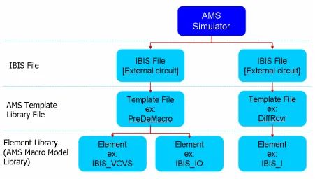
2.3 The IBIS-AMS Macro-model Hierarchy
The current, complete IBIS macro library components are listed in Appendix B. The
hierarchy is defined as follows [7],[10]:
Figure 2.3: AMS Hierarchy
The [external circuit] keyword would be in the IBIS file and would specify the AMS
Template file to be used. Please see the IBIS 4.1 specification [6] for more details. The
template files are predefined as part of the “template library”. For example, supposing we
wish to simulate a pre-emphasis buffer. Then the IBIS file would contain “[external circuit]
PreDeMacro.va” pointing the simulator to the template library file, PreDeMacro.va. The
PreDeMacro.va file would contain an AMS description of the pre-emphasis buffer by
instantiating Macro library elements (Appendix B) from the “element library”. A more
22
2.4 The Simulation algorithm
As shown in Chapter 1, an IBIS model contains several tables of data describing a
buffers behavior. An IBIS compatible simulator must make sense of this information so that
many load conditions may be simulated accurately using this limited behavioral description.
Each simulator has its own unique algorithm for approaching the issue so that simulation
time & accuracy are optimized. The algorithm used in the AMS library will be described in
this section. The implementation of the algorithm in an IBIS IO buffer model is provided in
Appendix E.
This algorithm makes use of the V-I curves (PullUp, PullDown, Power Clamp, GND
Clamp) to calculate the steady-state (DC) characteristics of the buffer. The Vt (Rising &
Falling waveforms) are used to calculate the transient behavior. This algorithm (& most
others) disregards the ramp rate. Due to backward compatibility the ramp rate is still
specified in IBIS files as part of the standard.
The algorithm uses the Vt curves to scale the PU & PD I-V curves with respect to
time to account for the partially on/off transistor characteristics during transients. The tables
that store these scaling values will be called the K* tables. The derivation of the K* tables are
described below.
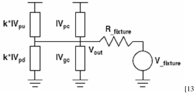
An output buffer is shown below. The IV* values denote each respective IV curve
[13]
Figure 2.4: IBIS Simulation Circuit
Assume that waveform1 and waveform2 are Rising Waveforms obtained with two different Vfixture values (usually VCC and GND). Since they are rising, the PU transistor will
be turning on while the PD transistor will be turning off.
The node equations for the above circuit will be as follows:
(
_ 1)
1(
_ 1)
10
=
K
pu on( )
t
•
IV
PU+
IV
PC−
K
pd off( )
t
•
IV
PD−
IV
GC−
I
out1( )
t
(
_ 2)
2(
_ 2)
20
=
K
pu on( )
t
•
IV
PU+
IV
PC−
K
pd off( )
t
•
IV
PD−
IV
GC−
I
out2( )
t
Where, out fixture out fixture
V
V
I
R
−
=
Since, typically, Vfixture1=0 & Vfixture2=Vcc (Requirement: Vfixture1< Vfixture2; for
easy programmability),
1
( )
( ) 0
( )
out out
out
fixture fixture
V
t
V
t
I
t
R
R
−
=
=
2( )
( )
out cc out
fixture
V
t
V
I
t
R
−
=
These two unknowns can be solved for each value of
t
using the two equations, 2 unknownsprocess.
These equations yield,
[
] [
]
(
) (
)
1 1 1 2 2 2
_
1 2 1
2
PD P
I
•
+
I
12
(
)
(
)
( )
out GC PC PC GC outpu on
PU PD PD PU
D
I
I
I
I
I
I
K
t
I
I
I
I
−
+
•
−
−
=
•
−
•
[
] [
]
(
) (
)
2 PUI
•
1+
1 1+
I
1 2−
2 2_
1 2 1 2
(
)
(
)
( )
out GC PC P PC GC outpd off
PU PD PD U
U
P
I
I
I
I
I
I
K
t
I
I
I
I
−
•
−
=
•
−
•
Similarly for the Falling Waveforms (where the PU transistor is turning off while the PD transistor is turning on):
[
] [
]
(
) (
)
1 1 1 2 2 2
_
1 2 1
2
PU P
I
•
+
I
12
(
)
(
)
( )
out GC PC PC GC outpd on
PU PD PD PU
U
I
I
I
I
I
I
K
t
I
I
I
I
−
+
•
−
−
=
•
−
•
[
] [
]
(
) (
)
2 PDI
•
1+
1 1+
I
1 2−
2 2_
1 2 1 2
(
)
(
)
( )
out GC PC P PC GC outpu off
PU PD PD U
D
P
I
I
I
I
I
I
K
t
I
I
I
I
−
•
−
=
•
−
•
Note that in this case (typically) Vfixture1=Vcc & Vfixture2=0. The requirement is that
Vfixture1> Vfixture2 for easy programmability.
The end results of all these calculations are the following arrays:
_
( )
pd on
K
t
,K
pd _off( )
t
,K
pu _ on( )
t
,K
pu _off( )
t
These arrays are computed once at simulation startup. When the simulation is in progress the
Going back to the original equations, for Rising and Falling cases respectively,
(
_)
(
_)
( )
( )
( )
out pu on PU PC pd off PD GC
I
t
=
K
t
•
IV
+
IV
−
K
t
•
IV
−
IV
(
_)
(
_)
( )
( )
( )
out pu off PU PC pd on PD GC
I
t
=
K
t
•
IV
+
IV
−
K
t
•
IV
−
IV
3. The IBIS-to-AMS converter
3.1 Introduction
As shown in the pre-emphasis buffer (above) example, the model maker customizes
the templates in the template library so that ‘real’ data is passed for simulation. Since the
templates are in Verilog or VHDL format, the next step is to use the IBIS to AMS converter
(GUI) script to convert raw IBIS files in to Verilog-AMS or VHDL-AMS format. The script
is listed in Appendix D.
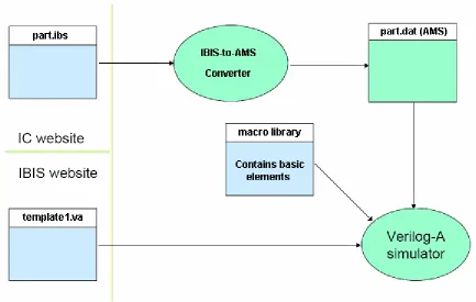
The customized template file, the AMS files created using the script, combined with
the macro library form the input set for the AMS simulator.
Figure 3.1: Simulation Process Diagram
The functionality of the script is explained in more detail in the following section.
3.2 The IBIS-to-AMS Flow
The ibis2ams.pl converter script was written in Perl/Tk. It can be obtained from the
IBIS-macro website. Converting IBIS files to AMS files involves using the ‘convert’ menu in
the GUI. The menu contents are as shown in the following figure.
Figure 3.2: ibis2ams Convert Manu
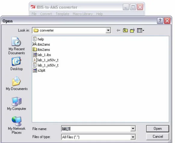
For example, consider the case where we want to convert the ‘io50v’ model (typical
corner) in lab_1.ibs to Verilog-AMS. The user would select ‘Convert IBIS file to Verilog-A’.
This would bring up the following dialog to select the input IBIS file.
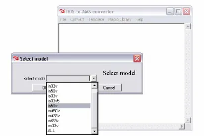
After the IBIS file is selected the following dialog queries the user to select the model
(in the IBIS file) that needs conversion. Note that selecting ‘ALL’ would convert all the
models (and corners) in the IBIS file to AMS. For this example, ‘io50v’ was selected.
Figure 3.4: ibis2ams Select model to convert
The next dialog asks the user to select the process corner (typical, minimum or
maximum) for data extraction.
Figure 3.5: ibis2ams Select process corner
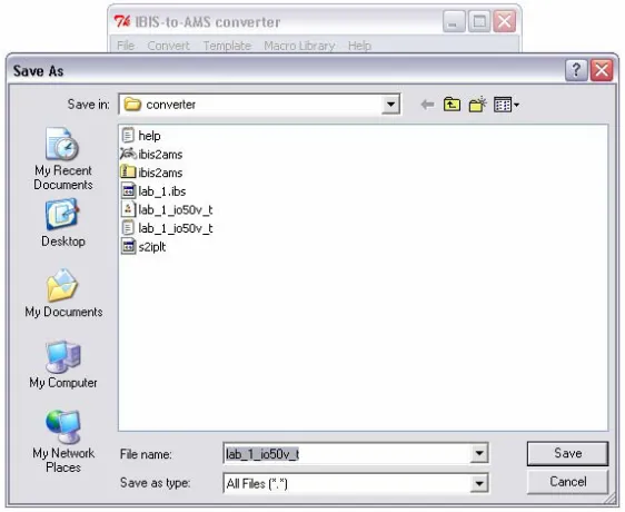
The next dialog asks the user to provide the AMS output file name. A default file
name is provided by the program with the following format:
<IBIS_file_name>_<Model_name>_<corner>.dat
Where <corner> is ‘t’ (typical), ‘n’ (minimum) or ‘x’ (maximum)
A part of the output Verilog-AMS file is shown below.
Figure 3.7: Sample Verilog-AMS output file
The VHDL-AMS file of the same model would look as follows.
32
4. Results
4.1 Introduction
Three case studies were performed to prove the accuracy, scalability and overall
viability of the methodology.
1. Output Buffer: A standard output buffer was simulated in hspice (transistor level) and
AMS and compared.
2. Pre-emphasis Buffer: This buffer can be described in traditional IBIS; however, the tap
delay would be hard coded. This example is based on the code written by Arpad Muranyi. He
had performed the simulation in Verilog-AMS; I translated the code to VHDL-AMS for
Dolphin SMASH compatibility.
3. Equalized Receiver: This buffer cannot be modeled in traditional IBIS. This example was
4.2 Case study I: Output Buffer
A standard output buffer that’s completely compatible with traditional IBIS will be used in
this example for proof of concept. The buffer is an Intel buffer provided by Michael Mirmak
and includes the pre-driver & all parasitics. The ESD diodes were removed due to lack of a
device model.
The flow used to create the AMS file describing the output buffer is given below. The
example will use SMASH VHDL-AMS as the simulation tool.
Figure 4.1 Conversion Flow
First, the Intel hspice netlist is converted to an IBIS file using the NCSU s2ibis utility. (All
the simulation files for this case study are provided in Appendix G)
Once the IBIS file is created, it must be converted to VHDL-AMS format using the ibis2ams
converter provided in Appendix D (and described in Chapter 3). This output file will be used
for the SMASH VHDL-AMS simulations.
The following circuit is simulated in SMASH. The instance X1 will be represented by the
VHDL-AMS file which was extracted above.
The SMASH GUI for the simulation is shown below:
Figure 4.3 SMASH GUI
The complete circuit description is given in the left plane. Notice the division between the
spice & VHDL sections. The Spice section describes the circuit given above and the VHDL
section defines the buffer sub-circuit (it also calls the VHDL-AMS data file which was
extracted). The right plane contains the simulator ‘use’ file which provides simulator
directives.
The results of the simulation are given below, plotted against the transistor level Hspice
results:
Figure 4.4 Output Comparison
The variation is clearly due to an underestimation of C_comp in the IBIS model. Note that
s2ibis doesn’t calculate C_comp. It simply defaults to 5pF leaving the model maker to tweak
the value. The matching between the transistor level hspice simulation & the SMASH AMS
simulation is quite good. The model-maker simply has to tweak the C_comp value to get a
36
4.3 Case study II: Pre-emphasis Buffer
A T-line (and package parasictics) presents LPF behavior. The high frequency
components are attenuated due to the T-lines physical characteristics. A high-frequency pulse
must have sufficient amplitude at the receiver for valid detection. The transmitter
equalization technique pre-emphasizes the high-frequency components of a signal and
minimizes the t-line attenuation problem. Pre-emphasis is done by means of a simple digital
filter. A single tap pre-emphasis buffer as the one shown below would have four static states,
depending on the states of the main & boost circuits. At a transition, both circuits are
switched on for one cycle to emphasize the rising or falling edge. At other points in time
where there is no transition the boost circuit remains off. Thus, its behavioral model would
have to keep track of previous data that is been input to the buffer. Modeling this device in
IBIS using current techniques would require the use of ‘tricks’ &/or the [driver schedule]
keyword making it a good candidate for macro-modeling. [12]
IBIS versions before 4.1 could not model a pre-emphasis buffer at all due to its output
dependency on previous output values. [driver schedule] was added in IBIS 4.1 but the
drawback was that the tap delay had to be hard coded in the IBIS file. Therefore, each time
the input clock frequency was varied, the user had to manually edit the IBIS file to reflect the
change in tap delay. Using the new methodology, the user can simply supply the delay as a
parameter through the main simulation file.
A schematic of the template is given below for ease of understanding. It can be seen that
the 2-tap pre-emphasis buffer template would have to contain the following elements:
1. An inverter
3. Four IBIS_OUTPUT (Appendix B) models for the drivers
4. Eight IBIS_I (current sources) to scale the boost buffers currents – The current
scaling for the boost circuit is achieved by scaling the supply currents provided to the
boost buffers. The eight supply nodes are: both (P & N) boost buffers pullup_ref,
powerclamp_ref, pulldown_ref & groundclamp_ref; hence the need for 8 current
sources.
Figure 4.5 Pre-emphasis Buffer Schematic
The VHDL-AMS template file which describes the Pre-emphasis buffer is provided
below. Note that the parameters ‘ScaleBoost’ and ‘TapDelay’ can be provided by the main
simulation file. Parameter passing in this manner provides a great deal of flexibility which
Figure 4.6 Pre-emphasis Buffer VHDL-AMS code (Part 1)
The following circuit was implemented in SMASH. The subcircuit X1 is described in
VHDL-AMS as shown above.
Figure 4.8 Pre-emphasis Buffer Test Circuit
The SMASH GUI is shown below.
Figure 4.9: Pre-emphasis Buffer SMASH GUI
The SMASH VHDL-AMS simulation results are shown below for an arbitrary input stream.
Depending on the value chosen for ‘ScaleBoost’, the tap will emphasize the signal at
switching points.
V(PLS)
V(OUTP)
V(OUTN)
4.4 Case study III: Equalized Receiver
The schematic of the receiver is shown below. This example doesn’t make use of IBIS data.
It simply provides a behavioral description of a differential input pair with receiver end
equalization and amplification.
Figure 4.11: Receiver Schematic
This receiver includes a passive equalizer and an amplifier. The equalization RC is
determined by Rpas & Cpas. Gain is equal to “(Rpas + Rt2) * gain/Rt2”
The VHDL-AMS code for the above circuit is given below. Note that the resistor, capacitor
and gain settings are all programmable.
The resultant waveform for an ideal differential input is provided below.
V(OUT) V(INP)
V(INN)
Figure 4.13: Receiver SMASH Output
The Transmission line model in SMASH isn’t complete yet, therefore I couldn’t
simulate a ‘real’ condition.
5. Conclusions & Future Research
5.1 Conclusions
As the operating frequencies & complexity of I/O buffers increased, many model
makers and/or users leave IBIS behind in favor of SPICE models; since IBIS is inaccurate or
unable to model these advanced buffers. Since most semiconductor vendors support their
models with a single vendor's version of SPICE, this trend brings the industry back towards a
single EDA vendor solution, which is what IBIS was designed to prevent. In an effort to
relinquish these shortcomings, in IBIS version 4.1, multi-lingual model extensions were
added to IBIS so that it could recognize Berkeley-SPICE, VHDL-AMS and Verilog-AMS
files.
A Macro model library was developed by the IBIS-macro committee to model state of the
art buffers by combining IBIS & AMS languages. Several templates were written to model
state of the art IO buffers which couldn’t be modeled by traditional IBIS. A GUI based tool
was developed (ibs2ams) and extensively tested to convert standard IBIS files into AMS
formats. Combining the Macro library, the conversion tool and templates, several simulations
were done to prove the methods accuracy, scalability and overall viability. As a byproduct,
we have a programmable IBIS simulator written in AMS which can be updated as we choose.
GUI tools were created in Perl/Tk for s2iplt (IBIS wave plotting utility) & s2ibis (Spice
46
5.2 Future Research
As mentioned in the conclusion section above, a result of this effort is that we end up
with a completely programmable IBIS simulator in AMS. One line of action is to attempt to
solve the SSN issues with IBIS. The first step would probably be to implement BIRD 95 in
the AMS library simulation algorithm [21].
Another line of action would be to create more template files; for LVDS, impedance
compensated buffers, true differential, buffers with deterministic jitter insertion, Decision
Feedback Equalization, FIR equalized receiver models etc. Running accuracy studies for the
REFERENCES
[1] Hall, Hall, McCall, "High speed Digital Systems Design", IEEE Press
[2] P. Fernando, "IBIS Modeling", Presentation at Analog Devices, Boston MA
[3] http://www.intel.com/technology/silicon/mooreslaw/
[4] M. Casamayor, "A first approach to IBIS models", Analog Devices Application note.
[5] http://www.freelists.org/archives/IBIS-macro/
[6] IBIS Version 4.1 (I/O Buffer Information Specification), January 2004
[7] Muranyi, “IBIS 4.1 Macros for simulator independent models”, DAC IBIS summit, June
2005.
[8] D. Telian, “Modeling complex I/O with IBIS 4.1”, IBIS summit, January 2005.
[9] NCSU s2ibis3 manual.
[10] Westerhoff, “IBIS 4.1 Macromodel Library for simulator independent modeling”,
Designcon East IBIS summit, September 2005.
[11] http://www.eetimes.com/news/design/columns/eda/showArticle.jhtml?articleID=17407954
[12] ECE733 class project, http://www4.ncsu.edu/~prfernan/Xtra_files/733%20proj2.doc
IBIS Modeling Cookbook v4.0, http://www.eda.org/pub/ibis/cookbook/cookbook-v4.pdf
[13] Arpad Muranyi, “Accuracy of IBIS models with reactive loads”, DesignCon 2006, Santa
Clara, CA
[14] Giacotto & Muranyi, “A VHDL-AMS buffer model using IBIS v3.2 data”,
DesignConEast 2003, Marlborough, MA
48
[16] Ian Dodd , “IBIS - Addressing Challenges in Behavior and Measurement”, DesignCon,
February 2006.
[17] Arpad Muranyi, “Introduction to the IBIS Macro Model Library”, DesignCon, February
2006.
[18] Todd Westerhoff, “Current Status - IBIS 4.1 Macro Library for Simulator Independent
Modeling”, DesignCon, February 2006.
[19] Michael Mirmak, “IBIS and Behavioral Modeling”, DesignCon, February 2006.
[20] Lance Wang and ZhangMin Zhong, “Using IBIS for SI Analysis”, Asian IBIS Summit,
Shenzhen, China, December 2005
[21] Yang, Park, et al, “Multi-buffer SSN Simulation using BIRD95”, DAC 2005, Anaheim,
50
Appendix A
IBIS Macro Library Elements
Basic Elements
Table A.1: Basic Elements
Fixed Voltage Controlled Current Controlled
R IBIS_R IBIS_VCR IBIS_CCR
L IBIS_L IBIS_VCL IBIS_CCL
C IBIS_C IBIS_VCC IBIS_CCC
Sources
Table A.2: Sources
Fixed Voltage
Controlled
Current Controlled
Voltage Controlled with Delay
Current Controlled with Delay Voltage
Source IBIS_V IBIS_VCVS IBIS_CCVS IBIS_VCVS_DELAY IBIS_CCVS_DELAY Current
Operators
Table A.3: Operators
Current Controlled
Current (with scaler)
Voltage Controlled Voltage (with scaler)
Adders IBIS_CCCS_SUM IBIS_VCVS_SUM
Multipliers IBIS_CCCS_MULT IBIS_VCVS_MULT
Dividers IBIS_CCCS_DIV IBIS_VCVS_DIV Voltage Controlled Current
(with scaler)
Current Controlled Voltage (with scaler)
Adders IBIS_VCCS_SUM IBIS_CCVS_SUM
Multipliers IBIS_VCCS_MULT IBIS_CCVS_MULT
Dividers IBIS_VCCS_DIV IBIS_CCVS_DIV
Active Devices
Table A.4: Active Devices
IBIS Input buffer IBIS_INPUT
IBIS Output buffer IBIS_OUTPUT
IBIS Input/Output buffer IBIS_IO
IBIS Tri-state buffer IBIS_3STATE
IBIS Open-sink buffer IBIS_OPENSINK
IBIS I/O Open-sink buffer IBIS_IO_OPENSINK
IBIS Open-source buffer IBIS_OPENSOURCE
IBIS I/O Open-source buffer IBIS_IO_OPENSOURCE
Other Models
Table A.5: Other Models
Inductive Coupler IBIS_K
52
Appendix B
IBIS to Verilog-A converter script
This script was written to convert standard IBIS files to AMS format.
#!/usr/local/bin/perl #
# Paul Fernando NCSU, IBIS-MACRO 01/17/2006 # [email protected]
#
# IBIS-to-VerilogA converter script v0.1 (GUI capabilities added) - 1/30/06
# IBIS-to-VerilogA converter script v0.2 (VHDL-A(MS) parsing added) - 2/1/06
# IBIS-to-VerilogA converter script v0.3 (windows "pwd" bug fixed) - 2/2/06
# IBIS-to-VerilogA converter script v0.4 (more bug fixes) - 2/3/06
# IBIS-to-VerilogA converter script v0.5 (Updated 'convert' to handle ALL models & corners) - 2/6/06
# IBIS-to-VerilogA converter script v0.6 (references/v_range, Rise/Fall waveform ordering) - 2/8/06
#
# This program is used to convert ibis file to verilog/vhdl A(MS) files. # This program requires Perl/Tk. http://www.perl.com/download.csp
# Note: only the "convert" menu works so far #
########################################################################## #######################
use Tk 800.000;
use subs qw/file_menuitems convert_menuitems template_menuitems lib_menuitems help_menuitems/; require Tk::BrowseEntry; require Tk::LabEntry; use Tk::DialogBox; use Tk::Dialog; use Tk::ErrorDialog; $Help_file="help.txt"; $default_IBIS_file="lab_1.ibs";
########## Create scroller_bar
my $mw = MainWindow->new(-title => "IBIS-to-AMS converter");
my $t = $mw->Scrolled("Text", -width => 50, -height => 20, -scrollbars => 'se',
-wrap => 'none')->pack(-expand => 1, -fill => 'both'); # scrollbars on south & east
########## Create the menubar
$mw->configure(-menu => my $menubar = $mw->Menu);
map {$menubar->cascade( -label => '~' . $_->[0], -menuitems => $_->[1] )} ['File', file_menuitems], # Each of these functions is defined below, in the next section
['Convert', convert_menuitems], # Each of these functions is defined below, in the next section
['Template', template_menuitems], # Each of these functions is defined below, in the next section
['Macro Library', lib_menuitems], # Each of these functions is defined below, in the next section
['Help', help_menuitems];
if ($^O eq 'MSWin32') {
$current_dir=`cd`; chomp($current_dir); $current_dir=$current_dir."\\";
my $syst = $menubar->cascade(-label => '~System'); my $dir = 'dir | sort | more';
$syst->command(
-label => $dir,
-command => sub {system $dir}, );
} else{
$current_dir=`pwd`; chomp($current_dir); $current_dir=$current_dir."/";
}
print "Running on $^O"."\n";
print "Current directory is $current_dir\n";
MainLoop; ########################################################################## ################# ########################################################################## ################# ########################################################################## ################# ########################################################################## #################
# File Menu
########################################################################## #######################
sub file_menuitems {
# Create the menu items for the File menu.
my($motif, $bisque) = (1, 0); my $new_image_format = 'png';
[
54
if($mw>Dialog(title=>'Exit?', text=>'Confirm exit', buttons=>['Exit', 'Return'], default_button=>'Return',
-bitmap=>'warning')
->Show eq "Exit") { &exit }}], ];
} # end file_menuitems
########################################################################## #################
# This function converts a model in a normal ibis file to AMS format ########################################################################## #######################
sub convert_menuitems {
# Create the menu items for the File menu.
my($motif, $bisque) = (1, 0); my $new_image_format = 'png';
[
['command', '~Convert IBIS file to Verilog-A', qw/-accelerator Ctrl-c/,
-command => sub{ &ibs_to_AMS("verilog");}],
['command', '~Convert IBIS file to VHDL-A', qw/-accelerator Ctrl-c/,
-command => sub{ &ibs_to_AMS("vhdl");}], ];
} # end convert_menuitems
########################################################################## #######################
# opens an AMS template file and links its data
########################################################################## #######################
sub template_menuitems {
# Create the menu items for the template menu
my($motif, $bisque) = (1, 0); my $new_image_format = 'png';
[
['command', 'Open ~template file', qw/-accelerator Ctrl-t/, -command => sub{
}], ];
} # end template_menuitems
########################################################################## #######################
# Read AMS macro library and list its contents
########################################################################## #######################
[
['command', '~List macro library modules', qw/-accelerator Ctrl-l/, -command => sub{
if
($in_va_file=$mw->getOpenFile(-initialfile=>"$current_dir"."IBIS_macro_library.va")) {
#$t->configure(-state => 'normal'); # disallows user typing #my $f1 = $t->Frame->pack(-side => 'top', -expand => 1, -fill =>'y');
# Read modules in Verilog-A macro library file
open( INFILEP, "< $in_va_file" ) or die "Can't open $in_va_file"; $temp_modules="";
while( $line=<INFILEP> ) {
if($line=~m/^(\s*)module\s+/i) { @words = split(/\s+/, $line);
push(@macro_lib_modules, $words[1]); print "$words[1]\n";
$temp_modules=$temp_modules."\n$words[1]";
} }
close INFILEP;
#my $be = $f1->Label(-text => "$temp_modules", -relief => 'groove', -width => 50)
# ->pack(-ipady => 5, -side => 'left'); }
}], ];
} # end lib_menuitems
########################################################################## #######################
# help
########################################################################## #######################
sub help_menuitems { [
['command', '~Help', qw/-accelerator Ctrl-h/, -command => sub{&Editor_module($Help_file)}],'',
['command', '~About', qw/-accelerator Ctrl-a/, -command => sub { my $db2=$mw->Dialog(-title=> "About", -text=>"IBIS to AMS Converter\nNCSU, IBIS-Macro 2006\nRunning on
$^O\n\nContact:\nprfernan\@ncsu.edu"."\n",
-buttons=>['Ok'], -default_button=> 'Ok', -bitmap=>'info')->Show();}],
]; }
########################################################################## #######################
# ibs_to_AMS - Oversees the ibis to AMS conversion
########################################################################## #######################
56
# Prompt for input ibis file
if
($in_ibs_file=$mw->getOpenFile(-initialfile=>"$current_dir"."$default_IBIS_file")) { # Reinitialize data stucts
&Reset_data_structs; $in_model_name_temp=""; @choices="";
# Read models(@choices) in ibis file
open( INFILEP, "< $in_ibs_file" ) or die "Can't open $in_ibs_file"; while( $line=<INFILEP> ) {
if($line=~m/^(\s*)\[Model\]\s+/i) { @words = split(/\s+/, $line); push(@choices, $words[1]);
} }
close INFILEP;
push(@choices, "ALL");
# Create dialog for model selection
my $db1=$mw->Dialog(-title=> "Select model", -text=>"Select model", -buttons=>['Ok', 'Cancel'], -default_button=> 'Ok');
$db1->BrowseEntry(-label => "Select model", -choices => \@choices, -variable => \$in_model_name_temp, -justify=>'right')
->pack(-ipady => 2, -side => 'bottom', -fill => 'both'); #$db->insert('end', "\n");
my $ans=$db1->Show();
if($ans eq "Ok" && $in_model_name_temp ne "" && $in_model_name_temp ne "ALL") {
$in_model_name=$in_model_name_temp;
# Parse input file name
$in_ibs_file1=$in_ibs_file; $in_ibs_file1=~s/.ibs//g; ($temp, $in_ibs_file1)=$in_ibs_file1=~m/(.*\/)(.*)$/;
# Dialog to get process corner, default: typical
my $db2=$mw>Dialog(title=> "Select Process corner", -text=>"Select Process corner",
buttons=>['Typical', 'Minimum', 'Maximum', 'ALL'], -default_button=> 'Typical');
my $ans2=$db2->Show();
if($ans2 eq 'Typical') { $corner="t"; $corner1="Typical"; &ibs_to_AMS_conversion($_[0]); &Reset_data_structs;}
elsif($ans2 eq 'Minimum') { $corner="n"; $corner1="Minimum"; &ibs_to_AMS_conversion($_[0]); &Reset_data_structs;}
elsif($ans2 eq 'Maximum') { $corner="x"; $corner1="Maximum"; &ibs_to_AMS_conversion($_[0]); &Reset_data_structs;}
elsif($ans2 eq 'ALL') {
$corner="t"; $corner1="Typical"; &ibs_to_AMS_conversion($_[0]); &Reset_data_structs; $corner="n"; $corner1="Minimum"; &ibs_to_AMS_conversion($_[0]); &Reset_data_structs; $corner="x"; $corner1="Maximum"; &ibs_to_AMS_conversion($_[0]); &Reset_data_structs;
elsif($ans eq "Ok" && $in_model_name_temp eq "ALL") { foreach $in_model_name (@choices) {
if($in_model_name ne "ALL" && $in_model_name ne "") { # Parse input file name
$in_ibs_file1=$in_ibs_file; $in_ibs_file1=~s/.ibs//g;
($temp,
$in_ibs_file1)=$in_ibs_file1=~m/(.*\/)(.*)$/;
$corner="t"; $corner1="Typical"; &ibs_to_AMS_conversion($_[0], "FORCE"); &Reset_data_structs; $corner="n"; $corner1="Minimum"; &ibs_to_AMS_conversion($_[0], "FORCE"); &Reset_data_structs; $corner="x"; $corner1="Maximum"; &ibs_to_AMS_conversion($_[0], "FORCE"); &Reset_data_structs;
} } } } } sub Reset_data_structs{ $input_state=""; $ibs_model_type="";
%ibs_Vpu_ref=""; %ibs_Vpd_ref=""; %ibs_Vpc_ref=""; %ibs_Vgc_ref=""; %ibs_V_tf=""; %ibs_T_tf=""; %ibs_V_tr=""; %ibs_T_tr="";
%ibs_vrange=(); %ibs_I_pc=""; %ibs_I_gc=""; %ibs_I_pu=""; %ibs_I_pd="";
$ibs_Vinh=""; $ibs_Vinl=""; $ibs_V_pc=""; $ibs_V_gc=""; $ibs_V_pu=""; $ibs_V_pd="";
}
sub ibs_to_AMS_conversion{
# Read ibis file and create data structs &create_datastructs($in_ibs_file); &sort_rising_falling_entries;
# depending on selection create Verilog or VHDL output file. if($_[0] eq "verilog") {
if($_[1] eq "FORCE") {
&create_verilog_output_file("$current_dir"."$in_ibs_file1"."_$in_mod el_name"."_$corner".".dat");
}
elsif($out_file=$mw->getSaveFile(-initialfile=>"$current_dir"."$in_ibs_file1"."_$in_model_name"."_$corner"." .dat")) {
&create_verilog_output_file($out_file); }
}
elsif($_[0] eq "vhdl") {
if($_[1] eq "FORCE") {
58
}
elsif($out_file=$mw->getSaveFile(-initialfile=>"$current_dir"."$in_ibs_file1"."_$in_model_name"."_$corner"." .txt")) {
&create_vhdl_output_file($out_file); }
}
#&Editor_module($out_file); # Open output file in text viewer
#&print_all_structs; # Prints all datastructures to screen }
sub sort_rising_falling_entries{
my $temp_Vfx_r; my $temp_Rfx_r; my $temp_TR_counter; my $temp_ibs_T_tr; my $temp_ibs_V_tr;
# If V_fixture min & max don't exist copy V_fixture to them if($Vfx_r{"1n"} eq "") {$Vfx_r{"1n"}=$Vfx_r{"1t"};}
if($Vfx_r{"2n"} eq "") {$Vfx_r{"2n"}=$Vfx_r{"2t"};} if($Vfx_f{"1n"} eq "") {$Vfx_f{"1n"}=$Vfx_f{"1t"};} if($Vfx_f{"2n"} eq "") {$Vfx_f{"2n"}=$Vfx_f{"2t"};} if($Vfx_r{"1x"} eq "") {$Vfx_r{"1x"}=$Vfx_r{"1t"};} if($Vfx_r{"2x"} eq "") {$Vfx_r{"2x"}=$Vfx_r{"2t"};} if($Vfx_f{"1x"} eq "") {$Vfx_f{"1x"}=$Vfx_f{"1t"};} if($Vfx_f{"2x"} eq "") {$Vfx_f{"2x"}=$Vfx_f{"2t"};}
# R1 must have the lower Vfx (of R1 and R2) # F1 must have the higher Vfx (of F1 and F2)
if($ibs_model_type1 ne "IBIS_OPENSINK" && $ibs_model_type1 ne "IBIS_IO_OPENSINK" && $ibs_model_type1 ne "IBIS_OPENSOURCE" && $ibs_model_type1 ne "IBIS_IO_OPENSOURCE") {
if($Vfx_r{"1".$corner}>$Vfx_r{"2".$corner}) { # swap the two #print "Swapped Rising WFs for model:$in_model_name type:$ibs_model_type1 corner:$corner\n";
$temp_Vfx_r =$Vfx_r{"1".$corner}; $temp_Rfx_r =$Rfx_r{"1"};
$temp_TR_counter=$TR_counter{"1"}; $temp_ibs_T_tr =$ibs_T_tr{"1"};
$temp_ibs_V_tr =$ibs_V_tr{$corner."1"};
$Vfx_r{"1".$corner} =$Vfx_r{"2".$corner}; $Rfx_r{"1"} =$Rfx_r{"2"};
$TR_counter{"1"} =$TR_counter{"2"}; $ibs_T_tr{"1"} =$ibs_T_tr{"2"};
$ibs_V_tr{$corner."1"}=$ibs_V_tr{$corner."2"};
$Vfx_r{"2".$corner} =$temp_Vfx_r; $Rfx_r{"2"} =$temp_Rfx_r;
$TR_counter{"2"} =$temp_TR_counter; $ibs_T_tr{"2"} =$temp_ibs_T_tr; $ibs_V_tr{$corner."2"}=$temp_ibs_V_tr;
}
$temp_Vfx_f =$Vfx_f{"1".$corner}; $temp_Rfx_f =$Rfx_f{"1"};
$temp_TF_counter=$TF_counter{"1"}; $temp_ibs_T_tf =$ibs_T_tf{"1"};
$temp_ibs_V_tf =$ibs_V_tf{$corner."1"};
$Vfx_f{"1".$corner} =$Vfx_f{"2".$corner}; $Rfx_f{"1"} =$Rfx_f{"2"};
$TF_counter{"1"} =$TF_counter{"2"}; $ibs_T_tf{"1"} =$ibs_T_tf{"2"};
$ibs_V_tf{$corner."1"}=$ibs_V_tf{$corner."2"};
$Vfx_f{"2".$corner} =$temp_Vfx_f; $Rfx_f{"2"} =$temp_Rfx_f;
$TF_counter{"2"} =$temp_TF_counter; $ibs_T_tf{"2"} =$temp_ibs_T_tf; $ibs_V_tf{$corner."2"}=$temp_ibs_V_tf;
} }
# If [... reference]s are not provided use [voltage range] instead. if($ibs_Vpu_ref{$corner} eq "") {
$ibs_Vpu_ref{$corner}=$ibs_vrange{$corner}; }