ABSTRACT
HILL, KEVIN A. Climate and Tropical Cyclones. (Under the direction of Dr. Gary Lackmann).
Part I of the work presented here investigates the impact of relative humidity on TC size in idealized WRF simulations. It is hypothesized that outer-core precipitation influences TC size, and therefore environmental factors that influence the amount of outer-core precipitation in turn influence TC size. Outer-core precipitation affects TC size through the diabatic generation of lower-tropospheric PV, which can amalgamate with the TC central PV tower or remain at radius. Four idealized high-resolution numerical simulations with the WRF model were performed in order to test the hypothesized sensitivity of TC size to environmental humidity. Differences in TC size between the runs were substantial, consistent with the hypothesis; several TC size metrics demonstrate this difference, including differences of a factor of 3 in the size of the RMW in the simulations.
During the simulation period, moisture fluxes led to similar moisture content in the boundary layer in all simulations, although large differences remained above the boundary layer and outside of the initial moist envelope. A close correspondence between the inward protrusion of the dry air and the formation of persistent precipitation was found, indicating that the presence of dry air was responsible for differences in simulated precipitation outside of the eyewall. PV budget analysis reveals that size differences can be linked to differences in precipitation in outer rainbands and associated diabatic production of lower tropospheric PV, which both were larger in the more moist simulations. Several feedback mechanisms serve to reinforce TC growth.
analysis of TC structure changes in a future climate. The high-resolution model output was used to investigate structural changes, and to explore the mechanism of future intensity changes.
Climate and Tropical Cyclones
by
Kevin Anthony Hill
A dissertation submitted to the Graduate Faculty of North Carolina State University
in partial fulfillment of the requirements for the degree of
Doctor of Philosophy
Marine, Earth, and Atmospheric Sciences
Raleigh, North Carolina August 2010
APPROVED BY:
__________________________ __________________________
Gary M. Lackmann Anantha R. Aiyyer
Chair of Advisory Committee
__________________________ __________________________
! ""! BIOGRAPHY
Kevin was born in Buffalo, NY on 11 November 1982, and graduated from Clarence High School in 2000. Kevin’s first fascination with meteorology was lake effect snow storms, which dump large amounts of snow in very isolated areas. During high school, Kevin learned that he had an aptitude for math and science, and upon arriving at The State University of New York at Brockport, he chose to major in meteorology and minor in math and statistics, while taking additional courses in physics and computer science in order to prepare for graduate school. Upon graduating from Brockport with a B.S. in Meteorology and a minor in mathematics and statistics, Kevin began graduate school in Atmospheric Science at NCSU under the advisement of Dr. Gary. M. Lackmann.
! """! ACKNOWLEDGEMENTS
Support for this research was received from the Department of Energy (DOE grant ER64448) and the National Science Foundation (NSF grant ATM-0334427) both awarded to North Carolina State University.
I would like to thank the members of my advisory committee, Drs. Gary Lackmann, Anantha Aiyyer, Frederick Semazzi, and Lian Xie for their insights and helpful suggestions. I would especially like to thank Dr. Gary Lackmann for his support, patience, and advisement over the years. I am very fortunate to have worked with him throughout my graduate education. I would also like to thank other members of the MEAS faculty, I cannot believe how much I have learned over the last 6 years and your courses have been a large part of that.
I have been fortunate to work with a great group of people in the Forecasting Lab (or whatever it is called now?), and I acknowledge its members (both past and present) for everything from collaboration on research and technical support to laughter and friendship.
! "#! TABLE OF CONTENTS
List of Tables ...ix
List of Figures ...x
1. Introduction and background 1.1 Overall motivation behind TC research...1
1.2 TCs and climate change...2
1.2.1 Evidence ...2
1.2.2 Research Objectives...3
1.2.3 Previous research...5
1.2.3.1 TC maximum intensity...5
1.2.3.2 The tropospheric response to increased greenhouse gas concentrations...7
1.2.3.3 Greenhouse gas induced temperature changes in GCMs...9
1.2.3.4 Tropical cyclone intensity studies...12
1.2.4 Summary...15
1.3 TC Size...15
1.3.1 Motivation...15
1.3.2 Research objectives and hypothesis...16
1.3.3 Observed sizes...16
1.3.4 Controls on TC size...17
! #! 2. Methodology
2.1 Tropical cyclone size...23
2.1.1 Model set-up and initial conditions...23
2.1.2 Potential vorticity techniques...26
2.1.3 Analysis techniques...27
2.1.3.1 Wind radii...27
2.2 Future TC intensity, rainfall, and structure...28
2.2.1 Current climate conditions...28
2.2.2 Creation of future climate environment...29
2.2.3 Idealized tropical cyclone characteristics...30
2.2.4 Numerical model TC simulations...30
2.2.4.1 Simulations with 6-km grid spacing...31
2.2.4.2 Simulations with 2-km grid spacing...32
2.2.5 Analysis techniques...33
2.2.5.1 Computation of mass weighted inflow, outflow...33
2.2.5.2 Comparison with MPI estimates...34
3. Tropical cyclone size 3.1 Simulated TC Intensity...41
3.2 Simulated TC Size...41
! #"!
3.4 Time evolution of water vapor fields...45
3.4.1 Simulation day 2 (hours 24 – 48)...45
3.4.2 Simulation day 8 (hours 168 – 192)...46
3.4.3 Summary of moisture changes...47
3.5 Physical mechanisms...48
3.5.1 Angular momentum import...48
3.5.2 Outer core precipitation, diabatic heating, and pressure gradient...49
3.5.3 Azimuthally averaged PV diagnostics...50
3.5.4 PV tower growth, eye and wind-field expansion...54
3.5.5 Spiral band structure...55
3.5.6 Feedback mechanisms...57
3.6 Summary...58
4. Future climate change and tropical cyclones 4.1 Future projections - TC environment...100
4.1.1 Environmental temperature...100
4.1.2 Environmental moisture...102
4.1.3 Large-scale conditions in sensitivity experiments...103
4.1.4 Freezing level and tropopause height...105
4.2 TC Intensity; thermodynamic efficiency and dynamical changes...106
! #""!
4.2.1.1 TC intensity...106
4.2.1.2 Thermodynamic efficiency...108
4.2.1.3 Dynamical influences: rainfall and PV...112
4.2.2 Simulations with 6-km grid spacing...116
4.2.2.1 TC intensity...116
4.2.2.2 Thermodynamic efficiency...117
4.2.2.3 Dynamical influences: rainfall...119
4.3 Structural analysis (2-km simulations)...120
4.3.1 Vertical velocity...121
4.3.2 Inflow...122
4.3.3 Outflow...123
4.3.4 Eye structure...123
4.4 TC Size...125
4.4.1 6-km Simulations...126
4.4.2 2-km simulations...126
4.5 Summary...127
5. Discussion and concluding remarks 5.1 TC Size...195
5.1.1 Additional implications and future research directions...198
! #"""!
! "$! LIST OF TABLES
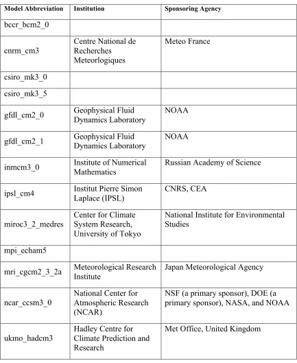
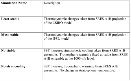
Table 2.1 Global climate models utilized in this study, along with the institution and agencies responsible for their development. In order to be used in this study, GCM output from the 20c3m, SRESA1B, SRESA2, and SRESB1 runs must have been available...36 Table 2.2 Summary of sensitivity experiments, and names that will be used to describe them in subsequent chapters...37 Table 4.1 Summary of projected changes in SST from the different emissions
scenarios...130 Table 4.2 Summary of simulated maximum intensity in 2-km simulations with ensemble mean projected climate changes, and MPI estimates. For the WRF simulations, the minimum values shown are the average of the minimum
values in the MYJ and YSU runs...131 Table 4.3 Summary of maximum intensity in 2-km simulations and sensitivity
! $! LIST OF FIGURES
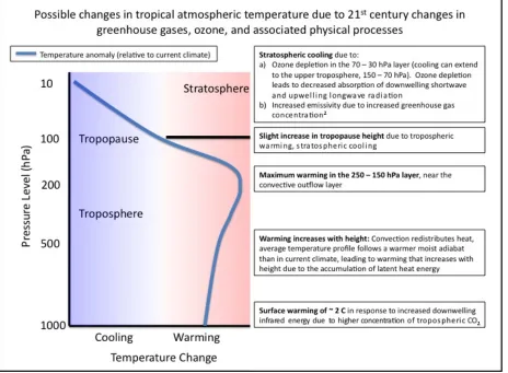
Figure 1.1 Schematic of GCM ensemble mean temperature change profile (blue curve) and the associated physical processes responsible for the change...22 Figure 2.1 Outline of region used for the averaging of environmental conditions in TC
size and future TC experiments. The region encompasses 8.5 – 15º North, and 60 – 40º West. ...38 Figure 2.2 Global GHG emissions (in GtCO2-eq per year) in the absence of additional
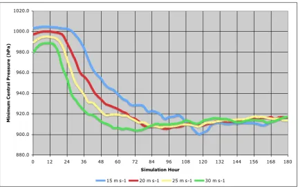
climate policies six illustrative SRES marker scenarios (colored lines) and 80th percentile range of recent scenarios published since SRES (post-SRES) (gray shaded area). Dashed lines show the full range of post SRES scenarios. The emissions include CO2, CH4, N2O, and F-gases. {WGIII 1.3, 3.2, Figure SPM.4] ...39 Figure 2.3 Time-series of minimum central pressure from WRF model simulations utilizing initial vortices of different strength blue (15 m s-1), red (20 m s-1), yellow (25 m s-1) and green (30 m s-1). 24-hour mean minimum central pressure values are 907, 907, 908, and 906 hPa for simulations with initial maximum winds of 15, 20, 25, and 30 m s-1, respectively...40 Figure 3.1 Time-series of simulated minimum central pressure (hPa)...61 Figure 3.2 As in Fig. 3.1 except maximum 10-m wind speed (m s-1)...62 Figure 3.3 Time-series of TC wind field parameters for each simulation as specified in legend, with application of a 1-2-1 smoother (a) radius of maximum 10-m wind speed (km); (b) maximum radius of hurricane-force 10-m wind speed. Values computed from azimuthally averaged model 10-m wind speed...63 Figure 3.4 Hovmöller diagram (with time on the ordinate and radius from TC center on
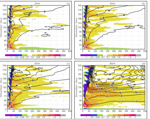
the abscissa) of azimuthally averaged 10-m wind speed (shaded; m s-1) for simulations (a) 20RH, (b) 40RH, (c) 60RH, (d) 80RH...64 Figure 3.5 Hovmöller diagram of the time rate of change of the azimuthally averaged
! $"!
Figure 3.7 As in Fig. 3.6, but for simulation hour 126...67
Figure 3.8 As in Fig. 3.6, but for simulation hour 180...68
Figure 3.9 As in Fig. 3.4 except for composite simulated radar reflectivity (dBz, shaded as in legend at bottom of panels). The radius of maximum 10-m wind speed, hurricane force wind, and tropical storm force wind are indicated by the black contours...69
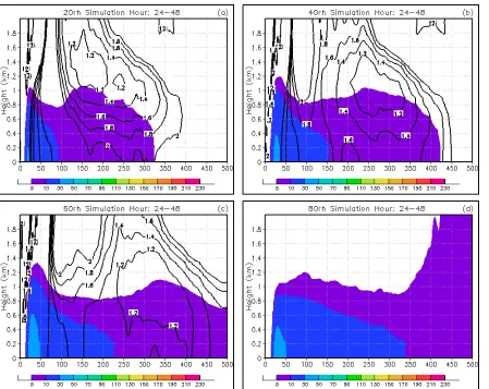
Figure 3.10 Cross-section of azimuthally averaged change (relative to initialization) in specific humidity (shaded; g kg-1) and specific humidity (contoured; g kg-1) time averaged between simulation hours 24 and 48...70
Figure 3.11 Cross-section of azimuthally averaged change (relative to initialization) in relative humidity (shaded; %) and relative humidity (contoured; %) time averaged between simulation hours 24 and 48...71
Figure 3.12 Cross-section of difference (relative to the 80RH simulation) in relative humidity (shaded; %), relative humidity (black contours; %), and the 15 dBz simulated radar reflectivity contour (red contour) time averaged between simulation hours 24 and 48...72
Figure 3.13 Cross-section of equivalent potential temperature (K; contoured) and the equivalent potential temperature lapse rate (K/km; shaded) time averaged between simulation hours 24 and 48...73
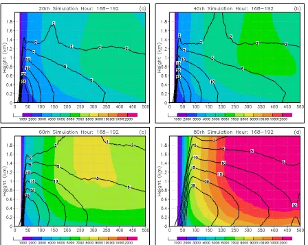
Figure 3.14 As in Fig. 3.10 except for between simulation hours 168 and 192...74
Figure 3.15 As in Fig. 3.11 except for between simulation hours 168 and 192...75
Figure 3.16 As in Fig. 3.12 except for between simulation hours 168 and 192...76
Figure 3.17 As in Fig. 3.13 except for between simulation hours 168 and 192...77
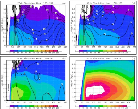
Figure 3.18 Cross-section of azimuthally averaged angular momentum (shaded; m2 s-2) and radial inflow (contoured; m s-1) time averaged between simulation hours 24 and 48...78
Figure 3.19 Cross-section of azimuthally averaged angular momentum multiplied by radial inflow (shaded; m3 s-3) and the value in the 80RH simulation divided by the value in that simulation (contoured), time averaged between simulation hours 24 and 48...79
Figure 3.20 As in Fig. 3.18 except for between simulation hours 168 and 192...80
! $""!
Figure 3.22 Tangential wind tendency (shaded; m s-1 hr -1) and angular momentum import (contoured). Data averaged over the lowest 2-km of the troposphere. ...82 Figure 3.23 850 – 700 hPa layer average latent heating (shaded; K hr-1) and composite
simulated reflectivity (contoured)...83 Figure 3.24 850 – 700 hPa layer average latent heating (shaded; K hr-1) and surface
pressure gradient (contoured)...84 Figure 3.25 Cross-section of azimuthally averaged potential vorticity (shaded; PVU),
simulated radar reflectivity (red contour; dBz) and potential temperature (black contours; K) time averaged between simulation hours 0 and 24...85 Figure 3.26 As in Fig. 3.25, except for time averaged between simulation hours 72 and 96...86 Figure 3.27 As in Fig. 3.25, except for time averaged between simulation hours 144 and
168...87 Figure 3.28 Azimuthally and layer-averaged 850-700 hPa PV (PVU, 1 PVU = 10-6 m2 s-1
K kg-1, shaded as in legend at bottom of panels, extending to 150-km radius). The radius of maximum 10-m wind speed is shown by the thick black line and 30 and 60 km radii are highlighted for reference...88 Figure 3.29 Azimuthally averaged composite reflectivity (shaded greater than 40 dBZ, as
in legends) and average 850-700 hPa PV (contoured, PVU) after 1 pass with a 9-pt smoother. The radius of maximum 10-m wind speed is shown by the thick black line and radii of 45 and 90 km are highlighted...89 Figure 3.30 Azimuthally and layer averaged 850-700 hPa diabatic PV tendency (shaded,
PVU hr-1) and PV (PVU, solid black contours). The radius of maximum 10-m wind speed is shown by the thick blue line and radii of 45 and 90 km are highlighted...90 Figure 3.31 As in Fig. 3.28, except extending to 500-km radius and highlighting smaller
PV values. Also, the radius of hurricane and tropical storm force wind are indicated by the thick black lines...91 Figure 3.32 As in Fig. 3.30, except extending to 500-km radius and highlighting smaller
PV values. Also, the radius of hurricane and tropical storm force wind are indicated by the thick blue lines...92 Figure 3.33 (a) Azimuthally averaged, model-output net moist diabatic tendency from
! $"""!
diabatic tendency; (c) as in (a) except for negative diabatic tendency; (d) non-advective PV tendency due to moist diabatic processes...93 Figure 3.34 24-hour mean volume-average (0-80km, surface-250 hPa) mass-weighted PV for the 80RH simulation (a) and 20RH simulation (b), and the corresponding hourly rate of change of average PV for the 80RH simulation (c) and 20RH simulation (d)...94 Figure 3.35 24-hour averages of eddy PV flux (m PVU s-1) in the 80-km radius ring for
the 80RH simulation (black) and 20RH simulation (gray)...95 Figure 3.36 Horizontal plots of model instantaneous rainfall rate (shaded, in hr-1) and
distance from TC center (contoured) for the 80RH simulation valid at simulation time a) hour 84, b) hour 109, c) hour 116 minute 50, d) hour 134...96 Figure 3.37 850 hPa PV (solid contours every 2 PVU) and model simulated composite reflectivity (shaded as in legend at left of figure) at hours 72 (a), and 102 (b) 80RH_Fix simulation...97 Figure 3.38 Zonal cross-section plots through band indicated in Fig. 3.37a (a)
model-output diabatic tendency (! 103 K s-1, shaded as in legend), radial circulation (vector, vertical component scaled by 25 ub s-1), 0°C isotherm (red line), and simulated radar reflectivity (light blue contours); (b) as in (a) except with absolute vorticity vectors instead of circulation, and PV (PVU, blue contours) instead of reflectivity. (c) PV (PVU, blue contours), diabatic PV flux vectors, moist diabatic PV tendency (shaded as in legend), and 0°C isotherm...98 Figure 3.39 Azimuthally averaged 850-hPa absolute vorticity (shaded) and surface latent heat flux (W m-2, solid black contours)...99 Figure 4.1 Ensemble mean projected change in temperature (K) for each emissions scenario...135 Figure 4.2 Projected change in temperature (K) for each of the 13 GCMs used from the
! $"#!
Figure 4.6 Ensemble mean projected change in relative humidity (%) for each emissions scenario...140 Figure 4.7 Ensemble mean projected change in mixing ratio (g kg-1) for each emissions scenario...141 Figure 4.8 Projected change in mixing ratio (g kg-1) for each of the 13 GCMs used from the SRESA1B emissions scenario. Data table on the right provides mean, minimum, maximum, and standard deviation values at each pressure level...142 Figure 4.9 As in Fig. 4.8, except for the SRESA2 emissions scenario...143 Figure 4.10 As in Fig. 4.8, except for the SRESB1 emissions scenario...144 Figure 4.11 Projected SST increase (K) versus maximum tropospheric moistening (g kg-1) for each of the GCMs...145 Figure 4.12 Projected temperature (K) changes in sensitivity experiments. Although SST
changes are not listed, they follow closely the projected temperature change at the 1000-mb level...146 Fig. 4.13 As in Fig. 4.12, except for mixing ratio (g kg-1)...147 Figure 4.14 Freezing level (left) and lapse-rate tropopause (identified as the height at which the lapse rate becomes less than 2 k km-1) at simulation hour 0...148 Figure 4.15 Time-series of simulated minimum central pressure (hPa) in the control (black) and with ensemble mean projected future climate changes (see legend)...149 Figure 4.16 As in Fig. 4.15, except for the SRESA1B future simulation and the sensitivity
experiments (see legend)...150 Figure 4.17 Cross sections of temperature difference between the future environment and
! $#!
Figure 4.21 Outward mass flux as a function of temperature in the control, the SRESA1B, and the sensitivity experiments...155 Figure 4.22 Rain-rate (in hr-1) averaged between simulation hours 216 and 240, for the
control and future simulations with ensemble mean projected changes (emissions scenario indicated in each image)...156 Figure 4.23 As in Fig. 4.22, except for the simulation with projected changes from the
SRESA1B ensemble, and in tropospheric stabilization sensitivity experiments...157 Figure 4.24 Percentage increase in average rainfall in future climate experiments relative
to the control simulation within 250-km of the TC center. Values were averaged between simulation hours 216 and 240...158 Figure 4.25 Area averaged (within 250-km of the TC center) percentage increases (relative to the control simulation) of various quantities (indicated by legend). Parameters other than rainfall were computed at the 700-hPa pressure level. Values were averaged between simulation hours 216 and 240...159 Figure 4.26 Contoured frequency diagram of hourly rainfall rate (in hr-1) as a function of
time in the control simulation and future simulations with ensemble mean projected changes. Grid cells within 500-km of the objectively determined TC center were used. In future simulations, contours from the control simulation are shown for reference...160 Figure 4.27 As in Fig. 4.26, except for in the SRESA1B future simulation and in the
sensitivity
experiments...161 Figure 4.28 Cross sections of time-averaged (simulation hours 216 – 240) potential
vorticity (PVU; shaded), potential temperature (K; black contours), and the 0-C isotherm (blue contour) for the following simulations control (upper left), SRESA1B (upper right), SRESA2 (lower left), and SRESB1 (lower right)...162 Figure 4.29 As in Fig. 4.28, except for the SRESA1B and sensitivity experiments...163 Figure 4.30 Scatter plot of (top left panel) percentage increase in area-averaged (within
! $#"!
Figure 4.31 Central pressure reduction in future simulations (relative to control; central pressure deficit defined relative to the ambient environment) for future simulations with projected changes from individual GCMs driven by the SRESA1B emissions scenario...165 Figure 4.32 As in Fig. 4.31, except for projected changes from the SRESA2 emissions
scenario...166 Figure 4.33 As in Fig. 4.31, except for projected changes from the SRESB1 emissions
scenario...167 Figure 4.34 As in Fig. 4.31, except for projected changes from all emissions
scenarios...168 Figure 4.35 Simulated minimum central pressure versus MPI estimates (hPa). Simulations
with the YSU (red) and MYJ (blue) parameterization schemes are shown separately in order to highlight the differences. Separate linear regression lines and best fit parameters are also indicated...169 Figure 4.36 Left minimum central pressure (hPa) versus thermodynamic efficiency in all
78 future simulations with 6-km grid spacing. Right as in the left panel, but y-axis displays the thermodynamic efficiency multiplied by the SST...170 Figure 4.37 Left relationship between SST and mass-weighted inflow temperature (°C) in
all 78 future simulations with 6-km grid spacing. Right relationship between the increases (relative to control) in SST and inflow temperature (°C)...171 Figure 4.38 Left relationship between SST and mass-weighted outflow temperature (°C)
in all 78 future simulations with 6-km grid spacing. Right relationship between the increases (relative to control) in SST and inflow temperature (°C)...172 Figure 4.39 Percentage increase in area averaged rainfall in future simulations (relative to
control) all 78 future simulations with 6-km grid spacing...173 Figure 4.40 As in Fig. 4.39, except separated for each PBL scheme...174 Figure 4.41 Contoured frequency by altitude diagram of vertical velocity (m s-1) in the
control simulation and future simulations with ensemble mean projected changes...175 Figure 4.42 As in Fig. 4.41, except for the SRESA1B future simulation and the sensitivity
! $#""!
Figure 4.43 Contoured frequency by altitude diagram of inflow velocity (m s-1) in the control simulation and future simulations with ensemble mean projected changes...177 Figure 4.44 As in Fig. 4.43, except for the SRESA1B future simulation and the sensitivity
experiments...178 Figure 4.45 Contoured frequency by altitude diagram of outflow velocity (m s-1) in the
control simulation and future simulations with ensemble mean projected changes...179 Figure 4.46 As in Fig. 4.45, except for the SRESA1B future simulation and the sensitivity
experiments...180 Figure 4.47 Time (ordinate) – height (abscissa) plot of eye temperature anomaly (shaded;
°C) and vertical velocity (black contours; cm s-1). The dashed black contours indicate the eye subsidence (cm s-1) and the dashed line represents the thermal tropopause, where the lapse rate becomes less than 2 K km-1. The “eye” is defined as the 5 grid cells located within 2-km of the TC center, although the results are not sensitive to this choice...181 Figure 4.48 As in Fig. 4.47, except for the SRESA1B simulation and the sensitivity
experiments...182 Figure 4.49 Time-height plot of eye temperature anomaly difference (°C; shaded, relative
! $#"""!
! "!
Chapter 1
Introduction and Background
1.1 Overall motivation behind TC research
According to studies of hurricane damage, tropical cyclones (TCs) are the costliest natural disasters in the United States (Pielke and Landsea, 1998). The cost associated damage from TCs has been enhanced in the last few decades by a significant increase in population growth in coastal and near coastal regions, and as a result the United States is now more vulnerable to TCs than ever before (e.g., Sheets 1990; Marks et al. 1998; Pielke et al. 2008). The 2004 and 2005 Atlantic hurricane seasons illustrate this vulnerability, with both seasons setting numerous records for TC damage (Franklin et al. 2006, Beven et al. 2008). The 2004 Atlantic hurricane season was among the most damaging on record, with the United States suffering a record $45 billion in property damage, enduring landfalls from five hurricanes. The 2005 season broke many of the records set during 2004, with property damage from one storm alone (Katrina, with a damage estimate of $81 billion) almost doubling that of the entire 2004 season.
! #! 1.2 TCs and climate change
1.2.1 Evidence
An increase in Atlantic TC activity since 1995 has been observed (Goldenberg et al. 2001; Klotzbach 2006), and studies by Emanuel (2005) and Webster et al. (2005) have suggested that there has been an increase in global TC intensity since the 1970s. While others have questioned the interpretation and quality of the data (Landsea et al. 2006), the observed increase in Atlantic main development region (MDR) sea surface temperature (SST) during the 21st century (e.g. Vecchi 2008) suggests the potential for more intense TCs, given the close association between observations of SST and maximum TC intensity in the North Atlantic basin (Demaria and Kaplan 1994).
While multidecadal fluctuations in North Atlantic SST have been observed (Goldenberg et al. 2001), Santer et al. (2006) have presented model-based evidence that the rising trend in the Atlantic MDR SST is too large to be explained by internal climate variability alone and that human-caused changes in greenhouse gases are the main driver of the 20th-century SST increase. The Intergovernmental Panel on Climate Change’s (IPCC’s) Fourth Assessment Report (AR4; Solomon et al. 2007) concluded that most of the observed global mean temperature increase since the mid-twentieth century is very likely (defined as a probability of >90%) due to anthropogenic increases in greenhouse gas concentrations. Both of these findings suggest that the observed SST increase is due at least in part to increases in greenhouse gases, and a continued increase in surface temperature (and SST) is projected by all general circulation models (GCMs) that employ increasing concentrations of carbon dioxide (CO2) in the 21st century (Solomon et al. 2007).
! $!
warming may leave coastal communities even more vulnerable to TC impacts in the coming years. Therefore, TC-associated damage and fatalities throughout the globe have the potential to increase during the 21st century as anthropogenic global warming and coastal vulnerability both increase. Based on this threat, it is imperative that the impact of future climate change on TCs be investigated using the best analysis tools currently available; this is the main goal of the present study, which will be described in further detail in subsequent sections.
1.2.2 Research Objectives
In a recent review paper, Knutson et al. (2010) succinctly summarized previous studies that investigated the impact of climate change on TCs. Several of these studies will be summarized in future sections, but first it is important to outline the current state of relevant research in order to understand the uniqueness of this study. Previous studies indicate a likely increase in TC intensity, although a large number of these previous studies were conducted with resolution that was too coarse to realistically simulated observed TC intensity. Mechanisms responsible for the increase in intensity were generally not identified, and few studies sought to analyze changes in TC structure.
! %!
shear, and we assume that even if there were a modest increase in monthly-mean wind shear (e.g. Vecchi and Soden, 2007), low shear periods would still occur.
Previous studies have sought to address some of the questions we pose, but this study will advance previous research in a number of ways:
1. A larger sample of current state-of-the-art GCM projections will be utilized to provide estimates of changes in environmental SST and tropospheric temperature and moisture due to global warming, and this larger ensemble should provide a more robust prediction of these changes. Individual GCM projections that depart considerably from the ensemble mean will also be utilized, and the role of tropospheric stabilization in altering TC intensity will be isolated with specifically designed model experiments.
2. This study will place an increased emphasis on the physical processes responsible for changes in TC intensity, structure and rainfall.
3. TCs will be simulated using higher resolution than in previous studies, allowing for the omission of cumulus parameterization (CP), which is required at larger grid lengths. This improved resolution and lack of CP will allow for more realistic simulation of TC intensity and structure, aiding in our goal to make a more direct link to TC processes, structural changes, and theory in order to better understand the physical mechanisms responsible for intensity change.
! &! 1.2.3 Previous research
To form the basis for studying climate change and TCs, it is necessary to understand the environmental factors that impact TC intensity, and also the physical basis behind greenhouse gases altering tropospheric and stratospheric temperature and their representation in GCMs. Also required, of course, is an examination of previous studies that have investigated this topic.
1.2.3.1 TC maximum intensity
In order to examine how climate change may alter TC intensity, it is first necessary to understand what controls maximum TC intensity. Numerous attempts (e.g. Miller 1958, Malkus and Riehl 1960, Emanuel 1986, 1988, 1995, and Holland 1997) have been made to compute an upper bound on TC intensity for given atmospheric and oceanic conditions; this upper bound is usually stated as either the minimum surface pressure or maximum near-surface wind speed that a TC could attain a given environment. Assumed in most these derivations is the absence of environmental factors known to inhibit TC intensification, including wind shear, upwelling, and land interactions. Due to the presence of these detrimental factors, in nature only a fraction of TCs reach their maximum potential intensity (MPI)1 (Emanuel 2000). At first glance the relatively small number of observed TCs
attaining their MPI may call into question the usefulness of utilizing MPI in the context of climate change. However, Emanuel (2000) showed that the cumulative distribution functions (CDFs) of storm lifetime maximum intensity, normalized by climatological potential intensity, were nearly linear, but storms achieving hurricane strength have CDFs of smaller slope than those achieving only tropical storm strength. This suggests that there is a nearly uniform probability that a TC will achieve any given intensity up to marginal hurricane strength, and a uniform but lower probability that it will achieve any intensity between !!!!!!!!!!!!!!!!!!!!!!!!!!!!!!!!!!!!!!!!!!!!!!!!!!!!!!!!
1Also of note is the fact that some observed TCs have exceeded the MPI (Montgomery et al. 2006), possibly due
! '!
marginal hurricane intensity and the potential intensity. In other words, based on current observations if global warming were to result in a 10 – 20% increase in MPI, the intensity of observed events would rise on average by the same percentage, including those TCs that do not attain their MPI. Therefore, an understanding of how MPI will change due to anthropogenic climate change may provide insight into how actual TC intensity will change as well.
Relatively recent analysis of different techniques for estimating MPI has revealed that the theory debuted in Emanuel (1986, hereafter referred to as EMPI), is the closest to providing a useful calculation of maximum intensity and that it also predicts a structure similar to that of observed TCs (Camp and Montgomery, 2001). Emanuel (1986) advanced the hypothesis that the intensification and maintenance of TCs depends exclusively on self-induced heat transfer from the ocean, and derived a relation between environmental parameters and TC maximum intensity. Two separate derivations were presented, the first based on a balance between frictional dissipation and energy production in the inflowing boundary layer, and the second in which TC energetic processes were described as a simple Carnot heat engine in which latent and sensible heat are extracted from the ocean at a temperature Tin and ultimately given up in the outflow at a temperature Tout. The EMPI is
proportional to the thermodynamic efficiency, (Tin - Tout)/Tin. This efficiency, multiplied by
the oceanic heat source, represents the production of energy that is used to overcome frictional dissipation. The results suggest that extremely intense cyclones would occur with SSTs substantially warmer or upper tropospheric temperatures much colder than at present. Anthropogenic climate change leads to changes in both SSTs and upper tropospheric temperatures in the tropics, and therefore an understanding of both is required to assess potential changes in TCs intensity.
! (!
intensity was investigated. Increasing the SST while maintaining a fixed vertical temperature profile always led to more intense TCs, as anticipated; this is consistent with MPI theory, as increased SSTs lead to warmer inflow and increased thermodynamic efficiency. Model simulations indicated that stabilization in the upper troposphere led to a reduction in TC intensity; this again is consistent with MPI theory, as upper tropospheric warming leads to a warmer outflow temperature and lower thermodynamic efficiency. Specifically, they found that without stabilization aloft the intensity increase associated with an SST increase of 2° C would double, while the intensity increase associated with a more modest SST increase (1.5° C) could be completely offset by an increase in upper-tropospheric temperature of 3 - 4° C. As stated by the authors and will be described subsequently, in the tropics SST and tropospheric stability are related, with GCM output indicating increases in both tropical SST and tropospheric stability in future climate projections. Increases in SST and tropospheric stabilization consistent with the GCM output led to model-attained TC intensity increases of 7–8 hPa. In the absence of the tropospheric stabilization, however, the same SST increase led to an intensity increase of approximately double this amount, indicating that stabilization of the troposphere partially offsets the increase in TC intensity that would occur due to SST increase alone. Therefore, based on the results of this study and also MPI theory, it is not only increases in SST that will impact future TC intensity changes but also warming of the upper troposphere.
1.2.3.2 The tropospheric response to increased greenhouse gas concentrations
! )!
In an atmosphere with higher CO2 concentrations, downwelling infrared radiation to
the surface increases, leading to increases in surface temperature (or over the ocean, SST). Changes in the SST over the tropics subsequently lead to tropospheric lapse rate changes. The principle mechanism by which the tropospheric lapse rate is modified by surface temperature change in the tropics is the vertical transfer of heat by convective processes (e.g. Rennick 1977). In the absence of large-scale circulations, the tropical atmosphere tends to adjust toward an equilibrium that results when the loss of energy to space by long-wave radiation is balanced by the transfer of latent and sensible energy from the surface to the boundary layer, and its redistribution throughout the atmosphere by deep moist convection. The upper tropospheric temperature structure that results from convective adjustment is sensitive to the surface temperature, and in the tropics as the surface temperature increases moist convection produces an increasingly stable temperature stratification. Convective adjustment can act directly only in regions of frequent precipitation, which also tend to be regions of high SST (e.g. Zhang 1993; Fu et al. 1994), although advection and dynamical adjustment (e.g. Sobel et al. 2002) spread the convective heating to convectively inactive regions as well.
Complicating this relatively simple picture is the feedback between tropospheric water vapor and surface temperature (hereafter referred to as the water vapor feedback). Water vapor is a greenhouse gas, and as such increases in its concentration in the troposphere lead to an increase in downwelling infrared radiation, which leads to subsequent changes in surface temperature. Model experiments designed to isolate the impact of this feedback indicate that a strongly positive water vapor feedback amplifies greenhouse warming by a factor of 1.6 relative to an experiment with this feedback disabled (Houghton et al. 1990).
! *!
found that cooling in the stratosphere (70 – 30 hPa) due to ozone depletion leads to reduced downwelling longwave radiation, and subsequently leads to cooling that extends to the upper troposphere (150 – 70 hPa). Regardless of future changes in stratospheric ozone concentrations, cooling of the stratosphere is likely to continue as greenhouse gas concentrations increase. In a review paper discussing stratospheric temperature trends, Ramaswamy et al. (2001), found that increases in greenhouse gases accounted for ~1/4th of the observed 1979 – 1990 cooling trend in the lower stratosphere. In the stratosphere an increase in greenhouse gas concentration enhances the thermal emissivity. Due to the increase in emissivity, assuming that the radiation absorbed by this layer remains fixed, to achieve equilibrium the same amount of energy has to be emitted at a lower temperature and the layer cools. The increase in thermal infrared absorptivity, conversely, leads to enhanced absorption of radiation emitted by the troposphere, leading to a warming tendency. The net result is a balance involving these processes that depends heavily on the absorption spectrum. For CO2 the main 15-µm absorption band is saturated over quite short distances, and
therefore the absorbed radiation originates from the cold upper troposphere. When the CO2
concentration is increased, the increase in absorbed radiation is quite small and the effect of the increased emission dominates, leading to a cooling at all heights in the stratosphere. To summarize, temperature changes in the stratosphere impact the upper troposphere, and therefore model representation of stratospheric processes is important as it could potentially impact TC outflow and thermodynamic efficiency.
1.2.3.3 Greenhouse gas induced temperature changes in GCMs
! "+!
Cumulus parameterization (CP) schemes are generally classified as being either an adjustment scheme or a mass flux scheme. Adjustment schemes are active if a grid point is conditionally unstable and serve to relax the temperature profile to that of a reference profile, immediately precipitating out any water mass condensed by this procedure. Mass flux schemes are triggered by the presence of grid convective instability at a grid point, the existence of grid-scale mass convergence beyond some threshold, or exceedance of a threshold rate of destabilization at a grid point, and attempt to explicitly model feedback processes in each grid cell. Mass flux schemes generally provide a more accurate parameterization, including the magnitude of the vertical motion inside the clouds and the precipitation type and distribution. Grid length also plays a role in the accuracy of CP.
GCM projections are sensitive to the type of CP scheme employed, as described in Allan et al. (2002). A comparison of climate models revealed that the use of an adjustment scheme led to an upper troposphere that was too cold and dry, a common characteristic of adjustment schemes (e.g., Hack 1994), while temperature and moisture in the upper troposphere were more realistically simulated with a mass flux scheme. Specifically, Hack (1994) attributes the improvement in upper tropospheric temperature and moisture in models using mass flux schemes to the explicit vertical eddy heat transport term, which is not accounted for in adjustment schemes. The choice of scheme impacts the water vapor feedback, with mass flux schemes tending to transport water vapor more efficiently into the upper atmosphere, leading to a stronger dependence of temperature and moisture on changes in the surface temperature in models with mass flux schemes. Vertical resolution also impacts the performance of a CP scheme, as demonstrated by Tompkins and Emanuel (2000). In this study column models were run to an equilibrium state and the sensitivity to vertical resolution was analyzed. Convergence of the results was found with a uniform vertical resolution of 25 hPa, while coarser resolution led to significant errors in both the water vapor and temperature profiles (relative to the high resolution results).
! ""!
on upper tropospheric temperatures, and compare 20th century temperature trends from GCMs utilized in the IPCC AR4 to both observations and the NCEP reanalysis. Near the surface and through the middle troposphere the models agree reasonably well with each other and were generally within 2-3° C of the NCEP reanalysis. The model spread increases with height, as does the disagreement between observations and the models. Observations indicate a cooling trend in radiosonde observations down to 200 hPa, while the models exhibit a moist-adiabatic response in this region, indicating that convective processes have a dominant influence on temperatures at this level. Of the 19 models that were studied, all include well-mixed greenhouse gas forcing while only 11 include stratospheric ozone depletion. Models that include ozone depletion were found to be significantly closer to observations than the models that omit ozone variations. From the surface to 200 hPa, models including ozone depletion were found to be within the range of uncertainty for the radiosonde observations, while in the models without ozone depletion temperatures were within the range of uncertainly from the surface to only the 500-hPa level. These results indicate that model ozone concentrations impact temperature values into the troposphere, and that realistic ozone concentrations and representation of stratospheric processes are required to realistically simulate temperatures in the mid-upper troposphere.
! "#!
mean (as described in chapter 2), in order to provide a projection of the most likely change in TC intensity along with a measure of the uncertainty.
1.2.3.4 Tropical cyclone intensity studies
Studies investigating the impact of global warming on TC intensity have employed several different strategies. The most basic type utilizes a GCM to simulate past TC activity using observed SSTs (varying in time or based on a long-term climatology), and compares the results to TC activity in a future projection. By comparing TC activity from the future and current periods, changes in intensity, frequency, and other characteristics can be studied, and generally speaking systematic biases in the GCM should ideally cancel out. Due to the large computational expense associated with long-term integrations, GCMs are required to use horizontal resolution that is unable to realistically simulate important storm-scale physical processes that determine TC intensity (e.g., storm-scale variations in turbulent fluxes, secondary circulation, and eye-eyewall processes), in part stemming from the need to parameterize sub-grid scale convection. The CP scheme degrades the realism of the TC secondary circulation, impacting TC intensity as well (e.g., Davis and Bosart 2002). Due to these limitations, tropical disturbances in these models are often referred to as being “TC-like” in that the modeled storms are larger in size and weaker than those observed. Recently, GCM projections with grid spacing of less than 30 km have provided evidence for increasing TC intensity in a warmed climate (e.g., Oouchi et al. 2006; Bengtsson et al. 2007); however still higher resolution is required to reproduce observed TC intensities. Bengtsson et al. (2007) specifically found that model projections with increased resolution predicted a larger increase in the frequency of intense TCs in the future climate, highlighting the need for high-resolution models, with explicit convection, in studies of TC intensity change in future climates.
! "$!
2004; Shen et al. 2000). In this approach, model simulations of an individual idealized TC embedded in a simplified large-scale environment with no other disturbances and no land are performed. Large-scale conditions, including SST, atmospheric moisture, temperature, and wind, can be based on observational analyses or model data. These large-scale conditions are typically averaged over time and space to represent the average conditions that support strong TCs. By utilizing large-scale conditions from a GCM projection, the impact of climate change on TCs can be determined. Due to the absence of external factors detrimental to TC intensity, this approach is better suited for the study of maximum TC intensity, and allows for the impact of specific changes in assumed parameters or in the large-scale environment to be analyzed in isolation. Knutson and Tuleya (1999) demonstrated the viability of this methodology by showing that simulated TC intensification in the future climate was similar using either high-resolution regional model simulations or the idealized downscaling technique.
! "%!
100-km of TC center was found in high-CO2 experiments relative to the control. Overall, the
simulated intensity increases in these studies were found to be fairly similar and robust, and large increases in TC rainfall were also noted.
Using dynamical downscaling approaches, numerical models utilizing observed SSTs and atmospheric reanalyses have been able to reproduce year-to-year variability in Atlantic hurricane counts for 1980–2006 (Knutson et al. 2007). In these simulations, the interior solution is nudged towards atmospheric reanalyses on larger spatial scales. Due to shorter integration lengths and a smaller domain, these simulations were run with substantially higher resolution (18-km grid spacing) than full GCM projections, but still contained a larger number of TCs and transient synoptic-scale conditions. A similar approach was later adopted by Knutson et al. (2008) to study the impact of climate change on Atlantic TC activity, with the mean atmospheric state (used by the interior nudging) and SSTs altered according to late twenty-first-century changes simulated by an ensemble of the WCRP CMIP3 models, under Intergovernmental Panel on Climate Change (IPCC) emissions scenario A1B. Although finding a reduction in the total number of tropical storms and hurricanes, these simulations indicate an increase in the frequency and intensity of the strongest hurricanes, and an increase in near-hurricane rainfall rates. Although these simulations were performed at fairly high resolution, Bender et al. (2010) extended the modeling approach by downscaling each individual model storm from the 18-km simulations, noting that the 18-km simulations are unable to reproduce the observed frequency of intense hurricanes. These higher resolution simulations indicate an increase in the number of category 4 and 5 hurricanes in the future climate. The authors note that the results are sensitive to the manner in which the late 21st century changes were calculated, and whether or not ensemble-mean or individual GCM data are utilized.
! "&!
this possible change will also be investigated here. Also, the increase in intensity was attributed to warming SST, while a reduction in intensity due to tropospheric stabilization and outflow warming was also noted. The authors did not attempt to assess the sensitivity of the results to the GCM chosen for projected climate changes.
1.2.4 Summary
To summarize, previous studies that investigated the impact of climate change on TCs have typically noted an increase in maximum TC intensity, along with an increase in rainfall. While several studies have described the sensitivity of the results to the GCM projected tropospheric warming (e.g., Knutson et al. 2004; Bender et al. 2010), in general this has not been a main focus.
1.3 TC Size
1.3.1 Motivation
! "'!
speeds within 200-km of the center. Dynamically, the vulnerability of a storm to vertical wind shear and dry environmental air may be related to its size, and the movement of large storms may differ from that of smaller ones due to more pronounced beta drift. Fovell et al. (2009) document sensitivity in the track of simulated TCs to choice of model microphysics scheme, and relate this to differences in the lateral extent of the wind field. Climate change may also lead to changes in TC size. Therefore, knowledge of the environmental and dynamical factors that determine TC size is relevant to the prediction of TC track, intensity, and impacts. Despite the importance of TC size, the physical mechanisms determining this have received limited attention in the scientific literature (e.g., Liu and Chan 2002).
1.3.2 Research objectives and hypothesis
The purpose of this research is to investigate the influence of environmental humidity on the lateral extent of the TC wind field. We hypothesize that the size of the TC wind field is related to the extent and intensity of outer spiral rainbands, which are in turn related to the environmental relative humidity. More moist environments support a larger amount of precipitation outside of the TC core, which leads to greater diabatic PV production there and a larger wind field. This PV, if given a favorable geometric structure, may amalgamate with the TC core, although its mere presence outside of the TC core leads to a larger wind field (e.g., Hill and Lackmann 2009). Dry environments lead to suppressed rainfall outside of the TC core, and a narrower PV distribution and wind field. This hypothesis was tested by conducting idealized experiments with the WRF model, which are designed to isolate the sensitivity of size to environmental moisture.
1.3.3 Observed sizes
! "(!
radius of maximum wind (RMW), and breadth of satellite-observed cloud shield. Tropical cyclones (TCs) are observed to vary considerably in size (e.g., Frank and Gray 1980; Merrill 1984; Weatherford and Gray 1988; Cocks and Gray 2002; Kimball and Mulekar 2004). Notable differences in size between basins have been noted, such as those between the northwest Pacific and West Indies (Frank and Gray 1980), and between the Western North Pacific and North Atlantic (Merrill 1984). Well-documented extremes range from Supertyphoon Tip (October 1979), which was characterized by a radial extent of gale-force winds (17 m/s) of ~1100 km (Dunnavan and Diercks, 1980), to Tropical Cyclone Tracy (December 1974), which featured peak winds near 65 m/s, yet gale-force winds extending only 50 km from the center (Bureau of Meteorology 1977). The corresponding area experiencing gale-force winds was less than 8,000 km2 for Tracy and over 3,800,000 km2 for Tip. Within the Atlantic basin TC size varies substantially as well, with an order of magnitude differences noted in the radius of tropical storm force wind in extreme cases (e.g., Kimball and Mulekar 2004; their Table 2).
1.3.4 Controls on TC size
In general, previous studies have found little correlation between TC intensity and size. Frank and Gray (1980) noted that the extent of the 15 m s-1 wind speed radius was quite variable for TCs of similar maximum intensity. Merrill (1984) calculated a correlation coefficient of only 0.28 between storm size (measured as the radius of outermost closed isobar) and intensity (defined as the maximum wind speed) using a large sample of storms for the North Atlantic and Pacific basins. Weatherford and Gray (1988) found a weak relationship (R2 = 0.23) between minimum central pressure and the radius of 15 m s-1 wind.
! ")!
Previous studies have also sought to correlate differences in TC size with environmental parameters. Observational data indicates that storm size varies with latitude (e.g., Merrill 1984; Cocks and Gray 2002; Kimball and Mulekar 2004) with a tendency for size increases as a TC moves poleward. Changes in angular momentum import with latitude were hypothesized by Merrill (1984) to account for changes in TC size resulting from latitudinal changes or changes in synoptic environment. Studies of the extratropical transition of TCs have noted, as did Merrill (1984), that the size of the TC wind field often increases during recurvature (e.g., Jones et al. 2003). A tendency for TC to peak in size during the month of September was noted by Kimball and Mulekar (2004), while a peak was found during late season storms in the Western North Pacific (Cocks and Gray 2002).
! "*!
1.3.5 Potential vorticity (PV), TC rainbands, and TC size
Following the papers of Hoskins et al. (1985) and Davis and Emanuel (1991), numerous studies have utilized the PV framework for the study of tropical cyclones (e.g., Jones et al. 2003, section 3b). These include studies of TC motion (e.g., Wu and Emanuel 1995a,b; Shapiro and Franklin 1999), formation and intensification (e.g., Molinari et al. 1998; Davis and Bosart 2001, 2002; Möller and Shapiro 2002), and circulation dynamics (Wang and Zhang 2003). Using a nonlinear balance relation, Wang and Zhang (2003) demonstrated that a large fraction of the TC circulation could be recovered from a PV inversion, with notable unbalanced flow in the lower inflow and upper-level outflow layers. In the study of TCs, important principles from a PV perspective are superposition and diabatic generation, as illustrated in Davis and Emanuel (1991, their Fig. 1). The superposition principle states that the net balanced circulation associated with multiple PV anomalies is the arithmetic addition of the individual balanced circulations. For example, Molinari et al. (1998) used this framework to examine trough interactions with Hurricane Opal, and Möller and Shapiro (2002) and Shapiro and Möller (2003) utilized this framework to investigate the role of asymmetries in the intensification of Hurricane Opal. Davis and Bosart (2001, 2002) appealed to a combination of diabatic PV production and superposition to explain the genesis of Hurricane Diana (1984).
From a PV perspective, the size of the balanced primary circulation in a TC is linked to the size and strength of three cyclonic PV anomalies associated with the storm. The most prominent PV feature is the interior cyclonic PV tower; in high-resolution simulations of strong TCs, this PV anomaly can exceed 100 PVU2 (e.g., Hausman et al. 2006). These
extreme PV values, more typical of those found far above the tropopause, are attributable to intense latent-heating gradients in the presence of very large cyclonic vorticity in the TC eyewall. Diabatic PV growth due to condensational heating is responsible for the aforementioned interior cyclonic PV maxima. As shown by Raymond (1992), Stoelinga
!!!!!!!!!!!!!!!!!!!!!!!!!!!!!!!!!!!!!!!!!!!!!!!!!!!!!!!!
! #+!
(1996) and others, the rate of diabatic PV generation is related to the projection of the heating gradient onto the absolute vorticity vector. Due to the decrease in cyclonic circulation with height in a warm-core vortex, the absolute vorticity vectors tilt outward with height, meaning that the maximum diabatic PV production should be found radially inward and beneath the location of maximum heating.
Additionally, the TC core is associated with an equivalent cyclonic PV anomaly due to the warm potential temperature anomaly at the surface in the center of the storm, which also contributes to the storm circulation. Even with constant surface air temperatures, the lower surface pressure in a TC core yields larger potential temperature values there. Warm surface potential temperature anomalies are equivalent to cyclonic PV anomalies (Bretherton 1966), and thus contribute to the cyclonic TC wind field.
! #"!
! ""!
! "#!
Chapter 2
Methodology
2.1 Tropical cyclone size
2.1.1 Model set-up and initial conditions
In order to investigate the impact of relative humidity on TC size, a set of model experiments designed to isolate this parameter was required. A method designed by the author was created to initialize a TC-like vortex within a tranquil ambient environment. This initialization procedure, referred to as a “quasi-idealized” approach, has the advantage over real-case simulations in that the role of moisture on TC size can be isolated. Four idealized simulations designed to investigate the sensitivity of TC size to environmental humidity were performed using version 2.2 of the Weather Research and Forecasting (WRF-ARW) model). In each simulation, the environmental temperature profile and SST were specified as the mean for the region 8.5–15°N, 40–60°W, during the month of September 2005 (region
shown in Fig. 2.1). Atmospheric variables were computed from Global Forecast System (GFS) analysis data, and the SST was derived from the Reynolds 0.5° analysis. The moisture
field, which is a function of distance from TC center, will be described in a subsequent section. The average SST in this region was 29.2°C, favorable for intense TC development.
This region and time were chosen in order to be consistent with conditions that are favorable for TC development, but experiments with other environmental soundings, such as that of Jordan (1958) produced similar results (not shown).
! "$!
, (1)
where r is the radius, rmaxthe radius of maximum wind, and Vmax the maximum wind. The
parameter b is related to the size of the vortex, and b = 0.33 in all experiments. Vertical structure is introduced to the horizontal wind field by multiplying Vt (r) by a function w (p)
that decreases with pressure above 850 hPa:
, (2)
where pm is the vertical level of maximum tangential wind, set to 850 hPa. The initial vortex
was centered at 11°N, although additional experiments reveal that the results are not sensitive to this choice (not shown). Based on the specified wind profile, temperature anomalies in the TC were computed assuming gradient thermal wind balance. Next, surface pressure was recomputed with the addition of the TC temperature anomalies, and finally the full height field was recomputed utilizing the surface pressure field along with the temperature field.
! "%!
the moist envelope was based upon the assumption that a typical TC would contain substantial water vapor out to a distance of approximately double the radius of maximum wind. Several additional experiments were performed in order to examine the sensitivity of the results to the inclusion and radius of the moist envelope. An experiment with 20% ambient relative humidity and a moist envelope radius of 50-km was also performed. The results were found to not be very sensitive to the radius of the moist envelope, although the smaller moist envelope did reduce the TC size slightly. Experiments in which relative humidity was initially set to 80, 60, 40 or 20% everywhere (including inside the vortex) were also performed, and the results are highly similar to those with a moist envelope surrounding the initial vortex. The main difference is that the dryer simulations take longer to intensify due to the time required for moistening of the inner core. Finally, the wide range in ambient relative humidity values was imposed in order to provide a robust test of sensitivity to this parameter rather than to specifically reflect conditions in nature; however, the 20RH simulation could be analogous to conditions near the Saharan air layer in the North Atlantic (e.g., Dunion and Velden 2004, their Fig. 2, Dunion and Marron 2008).
The idealized experiments were conducted using the full-physics advanced-research WRF (ARW) on an actual geophysical domain, but with the domain set to include only water. Model simulations were run for 10 days, which allowed the storm size to evolve sufficiently for the purposes of this study. These simulations utilized a high-resolution vortex tracking inner domain (508 ! 508 grid points with 2-km grid spacing) one-way nested
within an outer domain (400 ! 400 points with 6-km grid spacing). The 1016 ! 1016 km
! "&!
Model experiments were performed on both an f-plane and with full Coriolis force. The sensitivity of TC size to environmental moisture was consistent in both sets of experiments, although in model simulations with full Coriolis the TCs approached the NW edge of the outer 6-km domain towards the end of the simulation due to beta drift. By utilizing an f-plane valid at 11°N the TCs moved little during the 10-day simulation, assuring that the nested domain remained nearly centered in the outer domain and reducing the possible impact of the lateral boundaries. Therefore, results shown here are from the f-plane simulations, although the results are similar with each set of simulations.
Cumulus parameterization was omitted on both domains. The WSM 6-class scheme was used for the parameterization of microphysical processes (Hong and Lim 2006). The Mellor-Yamada-Janji! (MYJ) surface layer scheme (Janji! 2002), based on Monin-Obukhov similarity theory, was used with the MYJ boundary layer parameterization, based on Mellor-Yamada 2.5-level turbulence closure.
2.1.2 Potential vorticity techniques
Central to our hypothesis is the production of PV in TC spiral rain bands. In order to examine the PV distribution and production in the idealized experiments, we utilize the isobaric PV-tendency equation of Lackmann (2002):
(3)
where q is the Ertel PV, is the nonadvective PV flux,
and are the three- and two-dimensional gradient operators, respectively, is the
! "'!
features, the horizontal flux term was divided into azimuthal mean and perturbation components.
The diabatic PV tendency computation employs two different forms of : for fixed domains, the model-output diabatic temperature tendency from the microphysics scheme was used. Output from moving nests in WRF version 2.2 does not include the model-derived diabatic tendencies, necessitating the use of a parameterization from Emanuel et al. (1987) for condensational heating in the moving-nest simulations:
(4)
where and are the dry and moist-adiabatic lapse rates, respectively. The model-output
diabatic tendency is more complete, as it includes latent cooling as well as heating, but comparisons of PV budget terms using both diabatic formulations were qualitatively similar (not shown). The frictional contribution to the PV tendency is treated as a residual.
2.1.3 Analysis techniques
2.1.3.1 Wind radii
! "(!
winds were maximized, while the RHW and RTS were computed as the maximum distance at which the azimuthally averaged wind speed exceeded the hurricane and tropical storm force criteria, respectively.
2.2 Future TC intensity, rainfall, and structure
In order to examine changes in future TCs, simulations of idealized TCs in large-scale conditions consistent with current observed conditions and projected future conditions were performed, and the climate sensitivity was investigated. To this end, this research combines reanalysis and analysis data for current climate conditions, GCM projections for estimates of climate change, and high-resolution TC simulations in an attempt to quantify the impact of global warming on maximum TC intensity and TC structure. Each component of the methodology will be addressed in subsequent sections.
2.2.1 Current climate conditions
! ")!
(MDR) as specified in Vecchi and Soden (2007). Simulations utilizing the large-scale conditions from the reanalysis data will hereafter be referred to as the “control” experiments.
2.2.2 Creation of future climate environment
In order to construct future climate values, future changes were calculated using GCM output. GCM output used here is a subset of that produced in aid of the most recent report of the IPCC. These GCMs were run with greenhouse gas concentrations specified in accordance with a number of different scenarios, described in detail in the IPCC Special Report on Emissions Scenarios (SRES; 2002). These scenarios are designed to span a range of demographic, economic and technological driving forces of greenhouse gas emissions. As such, each emissions scenario is considered to be equally plausible, and for this study we will utilize 3 commonly used future greenhouse gas emissions scenarios: SRESA1B, SRESA2, and SRESB1. In order to maintain consistency, GCMs utilized in his study must contain all necessary data fields from these three future scenarios and also from the 20C3M experiment, which is designed to replicate 20th century conditions. The SRESA1B scenario follows the A1 storyline, which describes a future world of very rapid economic growth, global population that peaks in mid-century and declines thereafter, and the rapid introduction of new and more efficient technologies. The A1B scenario assumes a balance across increases in both fossil intensive and non-fossil energy sources. The A2 storyline and scenario describe a very heterogeneous world, with continuously increasing global population, regionally oriented economic development, and fragmented technological change. Finally, the B1 scenario describes a convergent world with a global population that peaks in mid-century and declines thereafter, with rapid changes in economic structures towards a service and information economy, with the introduction of clean and resource-efficient technologies. The resulting estimates of greenhouse gas emissions are displayed in Fig. 2.2; to summarize, the scenarios listed in order of increasing emissions (and concentrations) are SRESB1, SRESA1B, and SRESA2.