Nonparametric Kernel Estimation of Annual
Maximum Stream Flow Quantiles
Ani Shabri
Department of Mathematics, Faculty of Science
Universiti Teknologi Malaysia
81310 UTM Skudai, Johor, Malaysia
Abstract A nonparametric kernel methods is proposed and evaluated perfor-mance for estimating annual maximum stream flow quantiles. The bandwidth of the estimator is estimated by using an optimal technique and a cross-validation technique. Results obtained from a limited amount of real data from Malaysia show that quantiles estimated by nonparametric method using these techniques have small root mean square error and root mean absolute error. Based on corre-lation coefficient test shown that the nonparametric model approach is accurate, uniform and flexible alternatives to parametric models for flood frequency anal-ysis.
Keywords Bandwidth, cross-validation, kernel, correlation coefficient.
Abstrak Abstrak Kaedah Nonparametric Kernel dicadangkan dan dinilaikan perlaksanaannya dalam menganggar kuantil aliran tahunan maksimum. Pen-ganggar bagi bandwidth dianggarkan menggunakan teknik optimal dan ’cross-validation’. Hasil keputusan menggunakan data sebenar yang terhad dari Malay-sia, menunjukkan bahawa penganggar kuantil berdasarkan model nonparametric menggunakan kedua-dua teknik ini menghasilkan nilai punca min ralat kuasa dua dan punca min ralat mutlak yang kecil. Berdasarkan ujian pekali korelasi menunjukkan bahawa pendekatan model nonparametric adalah tepat, seragam dan ianya boleh dijadikan sebagai kaedah alternatif bagi model parametric dalam analisis frekuensi banjir.
Katakunci Bandwidth, ’cross-validation’, kernel, pekali korelasi.
1
Introduction
have been used to estimate flood flow frequencies from observed annual flood series. The general extreme value (GEV) distribution is recommended as a base model in the United Kingdom. After appraising many distributions, the U.S. Water resources Council (WRC), issued a series of Bulletins recommending the Log-Pearson Type III (LP3) a base method for use by all U.S. Federal Agencies [1]. While the most commonly used in Canada being the three parameter log-normal (LN3), the Generalized Extreme Value (GEV) and the log-Pearson III (LP3) [2].
Recently, nonparametric density estimation methods have gained popularity in a variety of field of science, including hydrology. This model has the advantage. The shapes of nonparametric density functions are directly determined by the data [3]. It is not requiring assumptions about the distribution of the population of interest [1] and the estimation of parameters (i.e. mean, variance and skew) are not needed. The parametric distributions are limited to certain shapes, however nonparametric densities can adapt to the often-irregular empirical distribution of random variables found in nature [3].
In the present study, the nonparametric kernel method was compared with the GEV, LNIII, GPA and EV1 distributions. The objective of the present study is to introduce and evaluate the performance of annual maximum series using nonparametric techniques and parametric distributions based on real data.
2
Nonparametric Frequency Analysis
The probability density function f(x) estimated by a nonparametric method is given by [2]
f(x) = 1
nh
n
X
j=1
K
x−x
j
h
(1)
where x1 to xn are the observations, K() is a kernel function, itself a probability density
function, andhis a bandwidth or smoothing factor to be estimated from the data. The following condition are impose on the kernel [2]:
Z
K(z)dz = 1 Z
zK(z)dz = 0 (2) Z
z2K(z)dz = C6= 0
where Cis the kernel variance.
The kernel distribution function is the integration of the density Eq. (1) from−∞tox
[2]:
F(x) = 1
n n X j=1 Kl
x−xj
h
(3)
where Kl(u) =R u
−∞K(w)dw.
the kernel distribution function is [2]
xT =F−1
1− 1
T
(4)
where F−1() represents the inverse ofF(). The value of x
T can be determined by solving
Eq. (3) numerically.
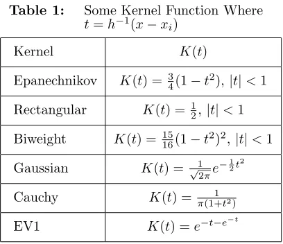
In nonparametric frequency analysis, the choice of kernel function is not critical since various kernels lead to comparable estimates [2]. Gaussian, Gumbel, and Epanechnikov kernels were tested in flood frequency analysis and it was found that the choice of the kernel does not important, and the shape of kernel does not affect extrapolation accuracy [2]. However the calculation and to choice of the bandwidth,hin Eq. 1 is critical. Table 1 shows some of the commonly kernels functions.
Table 1: Some Kernel Function Where
t=h−1(x−xi)
Kernel K(t)
Epanechnikov K(t) = 34(1−t2),|t|<1 Rectangular K(t) =12,|t|<1 Biweight K(t) =1516(1−t2)2,|t|<1 Gaussian K(t) = √1
2πe
−1 2t
2
Cauchy K(t) =π(1+1t2)
EV1 K(t) =e−t−e−t
In this study only the Gaussian kernel is considered.
3
Estimation Of Smoothing Factor
h
3.1
Optimal Technique (OPT)
Several bandwidth estimation techniques are based on minimization of an estimate of the mean square error (MSE) or of the IMSE function. IMSE is obtained by integrating the MSE function over the domain ofx.
The criterion of optimality is based on minimizing the IMSE given by [4]
IM SE= Z ∞
−∞ h
ˆ
f(x)−f(x)i 2
dx (5)
where ˆf(x) is an estimate of the known density function f(x). An optimal value of hcan be obtained by minimizing the IMSE for a given density f(x) and sample. The value of
determined numerically by differentiating the objective function Eq. (5) with respect to h
and then equating it to zero, is given by [4]
h= n X i=2 i−1 X j=1
(xi−xj) √
5n(n−10/3) (6)
Based on numerical studies have indicated that the computation of h is also optimal for small samples where n= 25 was the smallest sample considered [1].
3.2
Cross-Validation Technique (CV)
Other method of computing h is to minimize the integrated mean of a cross-validation technique [2]:
IM SE= Z ∞
−∞
Ehfˆ(x)−f(x)i2 dx
In cross-validation, estimates of f(x) are constructed each time using every data point except one. Let ˆf−i(x) be the nonparametric kernel estimate ignoring a single data point,
xi; that is
ˆ
f−i(x) =
1 (n−1)h
nX−1
j6=i
K[(x−xj)/h] (7)
The smoothing factorhcan be determined numerically from cross-validation procedure by solving Eq. (8) [2]
n
X
i=1,i=j n X j=1 exp d ij 4 (
1−4 √
2n n−1exp
d
ij
4
xi−xj
h
−1 !
xi−xj
h + 1
−1 )
= 0
(8) where dij = −((xi−xj)/h)2. The cross-validation procedure leads to consistent and
as-ymptotically optimal nonparametric density estimates.
4
Data Used For Numerical Analysis
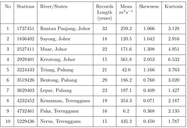
Table 2: Characteristic of Annual Maximum Stream Flow Data
No Stations River/States Records Mean Skewness Kurtosis Length m3s−1
(years)
1 1737451 Rantau Panjang, Johor 32 259.2 1.066 3.128
2 1836402 Sayong, Johor 18 120.5 1.042 2.916
3 2527411 Muar, Johor 22 171.6 1.308 4.951
4 2928401 Keratong, Johor 15 561.8 2.053 6.532
5 3224433 Triang, Pahang 21 42.0 1.166 3.763
6 3519426 Bentong, Pahang 29 186.2 0.760 3.020
7 3629403 Lepar, Pahang 23 197.1 0.409 1.427
8 4232452 Kemaman, Terengganu 19 354.3 0.071 2.187
9 4732461 Paka, Terengganu 16 6.2 0.368 2.135
10 5229436 Nerus, Terengganu 15 435.2 0.450 1.787
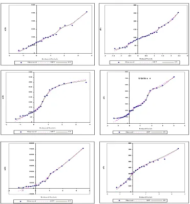
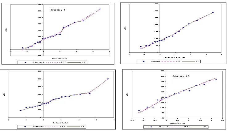
To assess how well the proposed nonparametric method fit to the observed annual maxi-mum flow data, theXT−T relationships using Eq. (4) are shown in Figure 1. The observed
flood discharge corresponds to a return period which was computed by using the Gringorton plotting position formula [5]
T = n+ 0.12
i−0.44 (9) in whichiis the rank assigned to each data point in the sample with a value of one the highest flow, two for the second highest and so on.
5
Results and Discussion
5.1
Root Mean Square Error And Root Mean Absolute Error
Two criteria were used for comparing the two methods of bandwidth h of nonparametric method. The first criteria is defined as the root mean square error (RMSE) between observed and computed flood discharge for entire sample. The RMSE is calculated by the equations
RM SE= v u u t1
n
n
X
i=1
xT −xˆT
xT
2
wherexT and ˆxT are observed and computed flood values, respectively for a given value of
T. The other criteria is the root mean absolute error and can be calculated by the equations
RM AE= v u u t1
n
n
X
i=1
xT−xˆT
xT
(11)
5.2
Goodness-Of-Fit Test
The goodness-of-fit test using correlation coefficient (CC) test is used to test the correlation,
r between the observations xT and computed flood value, ˆxT. The CC test is measure
of linearity of a probability plot. If the sample to be tested is actually drawn from the hypothesized distribution is expected to be nearly linear and the correlation coefficient will be near to one. If ¯xdenotes the average value of the observations and ¯wdenotes the average value of computed flood, then correlation coefficient sample can be defined as [6]
r= P
(xT −x¯)(ˆxT −w¯)
pP
(xT −x¯)2P(ˆxT −w¯)2
(12)
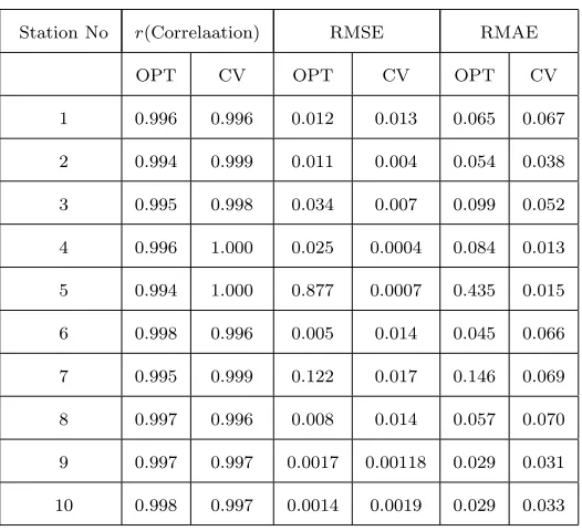
A comparison of the bandwidths for the Gaussian Kernel using OPT and CV for each stations is shown in Table 3.
Table 3: Comparison of Bandwidth for a Normal Kernel Base
on Values RMSE, RMAE andr
Station No r(Correlaation) RMSE RMAE
OPT CV OPT CV OPT CV
1 0.996 0.996 0.012 0.013 0.065 0.067
2 0.994 0.999 0.011 0.004 0.054 0.038
3 0.995 0.998 0.034 0.007 0.099 0.052
4 0.996 1.000 0.025 0.0004 0.084 0.013
5 0.994 1.000 0.877 0.0007 0.435 0.015
6 0.998 0.996 0.005 0.014 0.045 0.066
7 0.995 0.999 0.122 0.017 0.146 0.069
8 0.997 0.996 0.008 0.014 0.057 0.070
9 0.997 0.997 0.0017 0.00118 0.029 0.031
10 0.998 0.997 0.0014 0.0019 0.029 0.033
Figure 2: (Continue Figure 1)
The value of RMSE and RMAE for each stations using OPT and CV technique were presented in Figure 2. It can be seen that the value of RMSE and RMAE fall in nearly zero at all stations except at stations 5 and stations 7 for the OPT technique.
6
Conclusions
The correlation coefficient test statistic as a goodness of fit test is introduced for testing the nonparametric to fit the annual maximum flood flow data. The CC test statistic was found to be useful tool for discriminating among competing bandwidth estimation techniques. Overall these nonparametric method using the OPT and CV techniques consistently pro-duced linear probability plots with r nearly one as measured by the CC test statistics. The nonparametric models with these bandwidth estimation techniques are readily applicable to annual maximum flow frequency analysis.
Based on RMSE and RMSE, clearly, the CV technique is more accurate than the OP technique. However those differences between two methods were not too great and therefore these bandwidth techniques could be considered comparable for practical purpose.
It can be seen from the results presented here, that the nonparametric procedure is useful as it automatically gives stable and accurate estimates of density. It offers a practical and uniform approach to flood frequency analysis.
Acknowledgments
The author would like to thank the Department of Irrigation an Drainage in Malaysia for providing the flood flow data of streams in the Peninsular of Malaysia.
References
[1] K. Adamowski. A Monte Carlo Comparison of Parametric And Nonparametric Esti-mation of Flood Frequencies. Journal of Hydrology, 108(1989), 295-308.
[2] K. Adamowksi. Regional Analysis of Annual Maximum and Partial Duration Flood Data by Nonparametric and L-Moment Methods, Journal of Hydrology, 229(2000), 219-231.
[3] D. Faucher, P. F. Rasmussen & B. Bobee. A Distribution Function Based Bandwith Selection Method for Kernel Quantile Estiamtion. Journal of Hydrology, 250(2001), 1-11.
[4] S.L. Guo, R.K. Kachroo & R.J. Mngodo. Nonparametric Kernel Estimation of Low Quantiles, Journal of Hydrology, 185 (1996), 335-348.
[5] D. Jain & V.P. Singh. Estimating Parameters of EV1 Distribution For Flood Fre-quency Analysi, Water Res. Resources, 23(1987), 59-70.