A Comparison Of Plotting Formulas For The Pearson Type Iii Distribution

Jurnal Teknologi, 36(C) Jun. 2002: 61–74 © Universiti Teknologi Malaysia

A COMPARISON OF PLOTTING FORMULAS FOR THE PEARSON TYPE III DISTRIBUTION

ANI SHABRI*

Abstract. Unbiased plotting position formulas are discussed to fit the Pearson Type 3 distribution (PIII). The best quantile estimate made from the plotting position should be unbiased and should have the smallest root means square error among all such estimates. Probability plot correlation coefficient (PPCC) is used to evaluate goodness of fit to test the PIII distribution hypothesis. Results obtained using the annual maximum flow data from Peninsular of Malaysia based on PPCC show the plotting position formulas consistently produced linear probability plots with correlation coefficient near to one. Based on root mean square error (RMSE) and root mean absolute error, the Weibull formula performs better than the other formulas.

Keywords: Plotting Position, quantile, unbiased, root means square error

Abstrak. Formula kedudukan memplot tanpa bias dibincangkan untuk dipadankan dengan taburan Pearson 3 (PIII). Penganggar kuantil kedudukan memplot terbaik seharusnya tanpa bias dan mempunyai min punca ralat terkecil antara penganggar-penganggar yang lain. Pekali korelasi kedudukan memplot digunakan sebagai ujian pemadanan cocokan untuk menguji hi potesis taburan PIII. Hasil keputusan menggunakan data aliran maksimum daripada Semenanjung Malaysia berdasarkan ujian PPCC menunjukkan rumus kedudukan memplot menghasilkan plot kebarangkalian yang linear dengan pekali korelasi menghampiri satu. Berdasarkan punca min ralat kuasa dua dan punca min ralat mutlak, formula Weibull adalah terbaik antara formula-formula yang lain.

Kata Kunci Kedudukan Memplot, kuantil, tanpa bias, punca min ralat kuasa dua

1.0 INTRODUCTION

Probability plotting positions are used for the graphical display of annual maximum flood series and serve as estimates of the probability of exceedance of those series. Probability plots allow a visual examination of the adequacy of the fit provided by alternative parametric flood frequency models. They also provide a non-parametric means of forming an estimate of the data’s probability distribution by drawing a line by hand and or automated means through the plotted points. Because of these attrac-tive characteristics, the graphical approach has been favoured by many hydrologists and engineers. It has been widely used both in hydraulic engineering and water re-sources research [1, 3, 4 and 5].

*

Probability plotting positions have been discussed by hydrologists and statisticians for many years. To date, more than ten plotting position formule have appeared in the literature. Cunnane [2] and Stedinger et. al [7] published a very comprehensive review of the existing plotting formula. They postulated that a plotting formula should be unbiased and should have the smallest mean square error among all estimates.

Many distributions and various ways of fitting them are suitable. The selection distribution for any given flood records from among the alternative distributions is still a subject of continuing investigations. In hydrology many distributions for flood frequency analysis most often used, namely Extreme Value Type I (EV1), General extreme value (GEV), Pearson Type III (PIII), Log-Pearson Type III (LPIII), Log Normal (LNIII), General Pareto (GP), Wakeby and Weibull. Similarly, there are many plotting formula available, several of which are summarized in Table 1.

The choice of plotting position formula for fit to the distributions has been dis-cussed many times in hydrology and statistical literature. Different plotting positions attempt to use to achieve almost quantile-unbiasedness for different distributions. In this paper, the focus is to find the best plotting position formula to fit the PIII distribu-tion. In order to determine which plotting position formula is the most suitable for PIII distribution, the probability plot correlation coefficient test and RMSE and RMAE were used. The parameters for each distribution was estimated using moment method.

2.0 PEARSON TYPE III DISTRIBUTION

The Pearson Type III (PIII) distribution is used widely by hydrologists for modeling flood flow frequencies [5] and [8]. The Pearson type III probability density function may be expressed as

( )

_{( ) (}

(

)

)

= − −

Γ

1

α _ξ

β _{β ξ β}

α

x

f x x e ₍₁₎

where α, β and ξ are parameters. The parameters α, β and ξ are related to the first three moments of the random variable X as follows:

= + α µ ξ

β (2)

=

2 2 α σ

β (3)

= 2β_1/2 γ

β α (4)

3.0 THE INVERSE OF A PEARSON TYPE III DISTRIBUTION

( )

( )

( )

( )

∞

= >

= >

∫

∫

0

0 ξ

γ

γ x

x

F x f x dx

F x f x dx (5)

which given the complex form of f(x) in (1), is not easily inverted. Many investiga-tions have developed approximation inversion formula. Stedinger [7] found the good approximation for inverse of standardized PIII random variable is

= +µ σ

i i

p p

x K ₍₆₎

where K_piis referred to as frequency factor for the PIII distribution and can be written as

 

= _ + − _ −

 

3 2

2 2

1

6 36

γ _γ

γ i γ

i

p p

z

K ₍₇₎

where µ, σ and γ are mean, standard deviation and skew coefficient respectively, while z_pi is the p th quantile of the zero-mean and unit-variance standard normal distributions.

4.0 PLOTTING POSITION

Many investigators have advocated the use of quantile unbiased plotting positions when constructing probability plots. A quantile-unbiased plotting position is defined as [6]

( )

= _ _

i i

p F E X

where

[ ]

( )

i i

E X F p i n (8)

In situations where no historical floods are considered, most of them may be ex-pressed as a special case of general form

− =

+ −1 2

i

i a p

n a (9)

where p_i is the plotting probability of the i th order statistic, n is the sample size and a

for extreme value distribution (Hazen formula) and 3/8 for normal distribution (Blom formula)[7]. The approximation unbiased plotting position for PIII developed by Nguyen et. al takes the form [8]

− =

+ −

0.42 0.3γ 0.05 i

i p

n (10)

and is suitable for skews in the range − ≤ ≤3 γ 3 and samples in the range _{5≤ ≤n 100}. All of the plotting position formulas in this study are summarized in Table 1.

Table 1 Table 1 Table 1 Table 1

Table 1 Plotting Position Formulas (Cunnane, [2], Stedinger et al. [7]) Proponent

Proponent Proponent Proponent

Proponent FormulaFormulaFormulaFormulaFormula aaaaa Parent DistributionParent DistributionParent DistributionParent DistributionParent Distribution Weibull (1939) _ni₊₁ 0 All distributions

Beard (1943) i

n −

+ 0.3175

0.365 0.3175 All distributions

APL i

n −0.35

~0.35 Used with Probability Weighted Moments Method (PWM)

Blom (1958) _ni−₊3/8_1/4 0.375 Normal distributions

Cunnane (1977) i_n−₊0.40_0.2 0.40 GEV and PIII distributions

Gringorten (1963) i

n − +

0.44

0.12 0.44

Exponential, EV1 and GEV distributions Hazen (1914) i−_n0.5 0.50 Extreme Value distributions

Nguyen et.al (1989) _n+i_{0.3 + 0.05}−_γ0.42 PIII distribution

5.0 PROBABILITY PLOT CORRELATION COEFFICIENT TEST

A probability plot is defined as a graphical representation of the i th order statistic of the sample, x_i as a function of a plotting position. The i th order statistic is obtained by ranking the observed sample from the smallest (i = 1) to the largest (i = n) value, then

x_i equals the i th largest value.

A simple but powerful goodness-of-fit test is the probability plot correlation coeffi-cient (PPCC) test developed by Filliben in 1975, [7, 9]. The test uses the correlation r

between the ordered observations and the corresponding fitted quantilies

( )

i p

measure of linearity of a probability plot. If the sample to be tested is actually drawn from the hypothesized distribution, it is expected to be nearly linear and the correla-tion coefficient will be near to one. If x denotes the average value of the observations and w denotes the average value of the fitted quantiles, the correlation coefficient sample can then be defined as

(

)

(

)

(

)

(

)

i

i

i p

i p

x x x w

r

x x x w

− −

=

− −

∑

∑

The 5% critical values of PPCC test statistic of the PIII distribution can be approxi-mated using

( )

r_0.05 =exp 3.77 - 0.0290_ γ2 −0.000670n n_ 0.105γ−0.748 for γ ≤5 (12)

as given by Vogel et. al [8]. One rejects the hypothesized PIII distribution if the observed value, r, is smaller than the critical value.

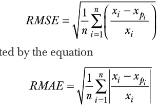
6.0 ROOT MEAN SQUARE ERROR AND ROOT MEAN ABSOLUTE ERROR

Root mean square errors (RMSE) and root mean absolute error (RMAE) are used to compare the efficiency of the different plotting positions formulas. The RMSE is calcu-lated by the equation

i n

i p

i i

x x

RMSE

n ₌ x

−

 

= _{ }

 

∑

1 1

(13)

while RMAE is calculated by the equation

i n

i p

i i

x x

RMAE

n ₌ x

−

=

_∑

1 1

(14)

where x_i and x_pi are observed and quantile values, respectively for a given value of i.

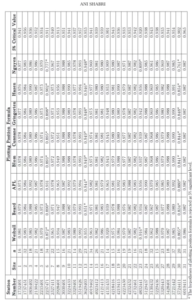
7.0 APPLICATION TO ANNUAL FLOOD DATA

Table 2

Correlation Coefficient Value (r ) of the Plotting Position Formulas and 5% Critical Value for the PIII Distribution

StationStationStationStationStation

Plotting Position FormulaPlotting Position FormulaPlotting Position FormulaPlotting Position FormulaPlotting Position Formula

NumberNumberNumberNumberNumber SiteSiteSiteSiteSite nnnnn WeibullWeibullWeibullWeibullWeibull BeardBeardBeardBeardBeard APLAPLAPLAPLAPL BlomBlomBlomBlomBlom CunnaneCunnaneCunnaneCunnaneCunnane GringortenGringortenGringortenGringortenGringorten HazenHazenHazenHazenHazen NguyenNguyenNguyenNguyenNguyen

5% Critical Value5% Critical Value5% Critical Value5% Critical Value5% Critical Value

1732401 1 1 6 0.981 0.979 0.975 0.978 0.978 0.977 0.976 0.977 0.941 1737451 2 3 2 0.983 0.984 0.984 0.984 0.984 0.984 0.984 0.983 0.956 1836402 3 1 8 0.985 0.988 0.992 0.989 0.989 0.989 0.990 0.986 0.936 2130422 4 2 1 0.982 0.985 0.987 0.986 0.986 0.986 0.987 0.986 0.952 2235401 5 1 8 0.970 0.973 0.978 0.974 0.974 0.975 0.975 0.970 0.934 2237471 6 3 4 0.872* 0.890* 0.931 0.893* 0.895* 0.898* 0.902* 0.777* 0.911 2527411 7 2 2 0.965 0.971 0.978 0.972 0.972 0.973 0.975 0.967 0.940 2928401 8 1 5 0.934 0.947 0.965 0.949 0.951 0.953 0.956 0.931 0.913 3030401 9 1 6 0.987 0.988 0.987 0.988 0.988 0.988 0.988 0.988 0.951 3224433 1 0 2 1 0.983 0.987 0.992 0.988 0.988 0.989 0.990 0.985 0.941 3329401 1 1 1 4 0.980 0.979 0.979 0.978 0.978 0.978 0.977 0.978 0.937 3519426 1 2 2 9 0.992 0.993 0.994 0.993 0.993 0.993 0.994 0.993 0.957 3629403 1 3 2 3 0.955 0.951* 0.944* 0.949* 0.949* 0.948* 0.946* 0.948* 0.955 4019462 1 4 3 4 0.963 0.971 0.982 0.973 0.974 0.975 0.977 0.960 0.941 4023412 1 5 2 6 0.982 0.981 0.981 0.981 0.981 0.981 0.980 0.981 0.959 4121413 1 6 2 1 0.986 0.983 0.979 0.982 0.981 0.981 0.980 0.980 0.959 4131453 1 7 1 4 0.920 0.939 0.965 0.943 0.945 0.948 0.953 0.909 0.901 4218416 1 8 1 5 0.975 0.978 0.981 0.979 0.980 0.980 0.981 0.980 0.943 4219415 1 9 1 6 0.984 0.988 0.992 0.988 0.989 0.989 0.990 0.987 0.936 4223450 2 0 1 9 0.970 0.976 0.983 0.977 0.977 0.978 0.979 0.971 0.933 4232452 2 1 1 9 0.987 0.987 0.988 0.987 0.987 0.987 0.987 0.987 0.953 4732461 2 2 1 6 0.982 0.982 0.983 0.982 0.982 0.982 0.982 0.982 0.942 4832441 2 3 2 5 0.916* 0.934 0.956 0.937 0.939 0.942 0.956 0.899* 0.920 5129437 2 4 1 8 0.984 0.987 0.990 0.987 0.987 0.988 0.988 0.985 0.938 5130432 2 5 3 2 0.962 0.967 0.970 0.968 0.968 0.969 0.969 0.961 0.943 5229436 2 6 1 5 0.988 0.987 0.985 0.986 0.986 0.986 0.985 0.986 0.938 5320443 2 7 2 3 0.970 0.977 0.985 0.979 0.979 0.980 0.982 0.969 0.935 5428401 2 8 1 8 0.987 0.988 0.989 0.988 0.988 0.988 0.988 0.987 0.941 5721442 2 9 3 7 0.985 0.989 0.992 0.990 0.990 0.990 0.991 0.985 0.954 5724411 3 0 2 0 0.805* 0.834* 0.880* 0.841* 0.844* 0.848* 0.854* 0.761* 0.902 6019411 3 1 3 1 0.986 0.987 0.987 0.987 0.987 0.987 0.987 0.987 0.965

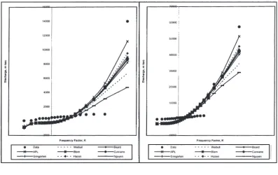
Figure 1 Comparison of Observed and Computed Frequency Curves For The 4 Stations With Difference r

(a) Station number 12, For r > 0.991 (b) Station number 6, With 0.776 < r < 0.932

β and ξ of the Pearson Type 3 distribution were estimated by using the method of moment.

Two criteria were used for comparing the eight plotting positions. The first criterion is defined as the probability plot goodness of fit. Table 2 shows the probability plot correlation coefficient, r, for 8 plotting position formulas and the 5% critical value of the PPCC test statistic using equation (11).

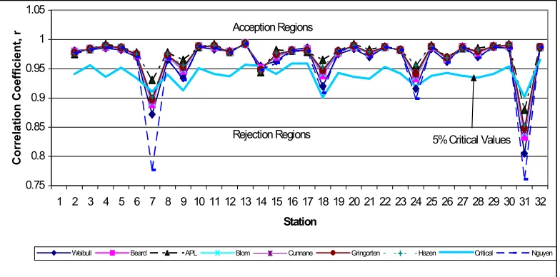
The correlation coefficient values of the plotting position formulas for each stations corresponding with 5% critical values are shown in Figure 1. Table 2 and Figure 1 show that the all plotting position formulas fall in accepted region at 5% critical values at all stations except the APL is rejected at two stations, Nguyen is rejected at four stations and the other formulas are rejected at three stations.

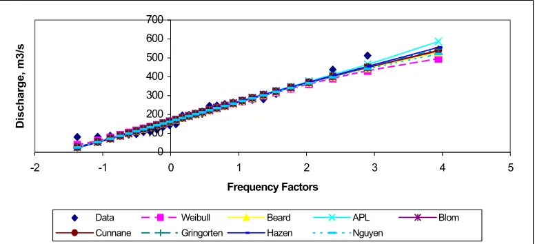
Two sets of observed data were selected for numerical demonstration. Figure 3 and Figure 4 show a demonstration comparison of plotting position formulas for r are accepted for station 12 and rejected for station 30 at 5% critical values. From Figure 3, it can seen that plots based on all of plotting position formulas are closed to data. However Figure 4 shows that the PIII using these plotting position formulas do not show good fit to the data especially at the largest data.

0.75 0.8 0.85 0.9 0.95 1 1.05

1 2 3 4 5 6 7 8 9 10 11 12 13 14 15 16 17 18 19 20 21 22 23 24 25 26 27 28 29 30 31 32

Station

Correlation Coefficient, r

Weibull Beard APL Blom Cunnane Gringorten Hazen Critical Nguyen Rejection Regions

Acception Regions

5% Critical Values

Figure 3 The Probability Plot Correlation Coefficient for the 8 Plotting Position Formulas and 5% Critical Values

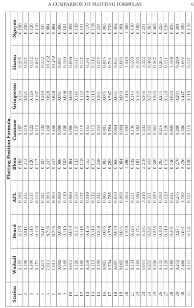
Table 3

Values of Root Means Square Error

Plotting Position Formula

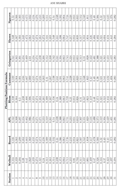
Table 4

Values of Root Means Absolute Error

Plotting Position Formula

The eight plotting position formulas were ranked for all stations according to the values of RMSE and RMAE on scale 1 to 8, with one being the best method.

0 100 200 300 400 500 600 700

-2 -1 0 1 2 3 4 5

Frequency Factors

Discharge, m3/s

Data Weibull Beard APL Blom Cunnane Gringorten Hazen Nguyen

-2000 0 2000 4000 6000 8000 10000 12000 14000 16000

-1 -0.5 0 0.5 1 1.5 2 2.5

Frequency Factors

Discharge, m3/s

Data Weibull Beard APL Blom Cunnane Gringorten Hazen Nguyen

Figure 4 Comparison of Observed and Quantile Using The Plotting Position Formulas (r Are Accepted At 5% Critical Values, Station 12)

Figure 5 Comparison of Observed and Quantile Using The Plotting Position Formulas (r Are Rejected At 5% Critical Values, Station 30)

Table 5 ranks the eight plotting position formulas according to RMSE. It can seen that the Weibull formula was the best, followed by APL, Beard, Blom, Cunnane, Gringorten, Nguyen and Hazen formulas in descending order of their performance.

Cunnane, Gringorten, Hazen and Nguyen formulas in descending order of their per-formance. Again, the previous conclusions hold. However those differences between plotting positions were not too great and therefore these plotting positions could be considered comparable for practical purpose.

Table 5 Ranking of the Plotting Position Formulas for 31 Stations by Root Means Square Error (RMSE) on a scale of 1 to 8 with 1 being the best method

Plotting

Position Number of Stations Receiving Ranking

1 2 3 4 5 6 7 8

Weibull 13 0 0 0 0 3 6 8

Beard 3 13 3 1 0 8 3 0

APL 10 3 7 3 2 3 2 1

Blom 2 2 8 9 10 0 0 0

Cunnane 2 0 4 15 10 0 0 0

Gringorten 0 6 6 0 5 8 4 1

Hazen 4 5 2 0 3 4 5 9

Nguyen 2 2 3 2 2 5 7 7

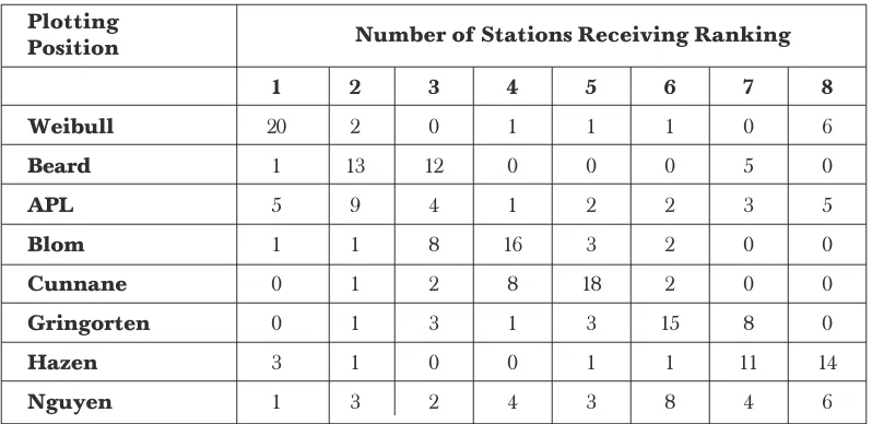
Table 6 Ranking of the Plotting Position Formulas for 31 Stations by Root Means Absolute Error (RMAE) on a scale of 1 to 8 with 1 being the best method

Plotting

Position Number of Stations Receiving Ranking

1 2 3 4 5 6 7 8

Weibull 20 2 0 1 1 1 0 6

Beard 1 13 12 0 0 0 5 0

APL 5 9 4 1 2 2 3 5

Blom 1 1 8 16 3 2 0 0

Cunnane 0 1 2 8 18 2 0 0

Gringorten 0 1 3 1 3 15 8 0

Hazen 3 1 0 0 1 1 11 14

8.0 CONCLUSIONS

Probability plots and the probability-plot correlation coefficient test statistic are used for testing the PIII using plotting position formula to fit annual maximum flow data. The PPCC test statistic was found to be a useful tool for discriminating among com-peting probability and plotting position formula. Eight plotting position formulas were compared for their ability to fit flood flow data. Overall these plotting position formu-las consistently produced linear probability plots with r nearly one as measured by the PPCC test statistics. If an unbiased plotting position formula is required for the PIII distribution, then the Weibull formula would be the best selection.

REFERENCES

[1] Adamowski, K. 1981. Plotting Formula For Flood Frequency, Water Resour. Bulletin, 17(2): 197-202. [2] C. Cunnane, C. 1978. Unbiased Plotting Positions- A Review, Journal of Hydrology. 37: 205-222. [3] Guo, S. L. 1990. A Discussion On Unbiased Plotting Positions For The General Extreme Value Distribution,

Journal of Hydrology. 121: 33-44.

[4] Guo, S. L. 1990. Unbiased Plotting Position Formula For Historical Floods, Journal of Hydrology. 121: 45-61. [5] Ji Xuewu, Ding Jing, H. W. Shen, and J. D.Salas. 1984. Plotting Positions For Pearson, Journal of Hydrology.

74: 1-29.

[6] Kottegoda N. T., and R. Rosso. 1997. Probability, Statistics, and Reliability for Civil and Environmental

Engineers. Mc-Graw Hill Book Co., New York.

[7] Stedinger, J. R., R. M. Vogel, and G. E. Foufoula. 1993. Frequency Analysis of Extreme Events. Handbook

of Applied Hydrology. Mc-Graw Hill Book Co., New York, Chapter 18.

[8] Vogel, R. M., and D. M. McMartin. 1991. Probability Plot Goodness-of-Fit and Skweness Estimation Procedures for the Pearson Type 3 Distribution, Water Resour. Res., 27(12): 3149-3158.