Raleigh, NC 27695-8203
Institute of Statistics Mimeo Series No. 2570
July 2004
Compactly Supported Radial Basis Function Kernels
Hao Helen Zhang Marc Geoton Peng Liu
Department of Statistics, North Carolina State University, Raleigh, NC hzhang, genton, [email protected]
Compactly Supported Radial Basis Function Kernels
Hao H. Zhang [email protected]
Department of Statistics
North Carolina State University Raleigh, NC 27695-8203, USA
Marc G. Genton [email protected]
Department of Statistics Texas A&M University
College Station, TX 77843-3143, USA
Peng Liu [email protected]
Department of Statistics
North Carolina State University Raleigh, NC 27695-8203, USA
Editor:
Abstract
The use of kernels is a key factor in the success of many classification algorithms by allow-ing nonlinear decision surfaces. Radial basis function (RBF) kernels are commonly used but generally associated with dense Gram matrices. We consider a mathematical opera-tor to sparsify any RBF kernel systematically. It yields a kernel with a compact support and sparse Gram matrix. Having many zero elements in Gram matrices can greatly re-duce computer storage requirements and the number of floating point operations needed in computation. This paper develops a unified framework to study the efficiency gain and information loss due to the sparsifying operation. We propose two quantitative measures: similarity and sparsity, and investigate their mathematical properties. Furthermore, the similarity-sparsity tradeoff is suggested to tune the thresholding parameter adaptively. We then implement compactly supported RBF kernels with tuning in support vector machines (SVM), least squares SVM, and kernel principal component analysis. Simulations demon-strate that properly-tuned compactly supported kernels give favorable performances while enjoying efficient algorithms for computation.
Keywords: Radial Basis Function, Sparse Gram Matrix, Support Vector Machines, Kernel Principal Component Analysis.
1. Introduction
For any input space X ⊂ Rd, a kernel is a positive definite function k : X × X → R, satisfyingPn
i,j=1aiajk(xi,xj)≥0 for anya1, ..., an∈Randx1, ...,xn∈ X. A kernel can be
regarded as a similarity measure between any two inputs. Gaussian kernels and polynomial kernels are commonly used; see Genton (2001) for a variety of kernels.
Given a training set of input vectors x1, ...,xn ∈ X, the Gram matrix associated with
a kernel k is an n×n matrix K with elements Kij = k(xi,xj) for i, j = 1, ..., n. K is
symmetric, positive definite, and generally dense in terms of not having any zero entries. A dense Gram matrix can be highly ill-conditioned especially for large datasets, thus posing severe numerical problems in solution feasibility and stability. Various methods have been proposed to speed up kernel machines, such as decomposition methods for SVM by Osuna et al. (1997), speedup methods for kernel PCA (Smola and Sch¨olkopf (2000), Smola et al. (2000)), and other kernel methods (Burges (1996), Williams and Seeger (2001)).
The motivation of our work is to construct kernels which have local support and sparse Gram matrices. A closely related work was developed in Achlioptas et al. (2002) which sparsifies the Gram matrixK by randomly omitting its entries with some sampling scheme. Our method is based on certain thresholding techniques. One straightforward idea is to re-place all small entries (smaller than some cutoff value) inK directly by zeros. However, this naive thresholding often destroys positive definiteness of the Gram matrix. In this paper, we study a mathematical operation which sparsifies K systematically while maintaining its positive definiteness. We will focus on radial basis function (RBF) kernels. Section 2 introduces compactly supported RBF kernels and discusses the efficiency gain in storage and computation with sparse Gram matrices. Section 3 proposes two quantitative mea-sures, similarity and sparsity, to characterize sparsified Gram matrices, and shows how the similarity-sparsity tradeoff can be used to tune the thresholding parameter adaptively. A practical solution for selecting the thresholding parameter is further provided for the special case when the memory required to store K is beyond computer capacity. Section 4 illus-trates the performances of compactly supported RBF kernels in three different contexts: support vector machines (SVM), least squares SVM, and kernel principal component anal-ysis (PCA). Section 5 shows two real world examples, one of which has a high dimensional input space. A discussion is given in Section 6.
2. Compactly Supported Kernels and Gram Matrices
In this section, we define compactly supported RBF kernels and study the sparse property of their Gram matrices.
2.1 Compactly Supported RBF Kernels
A radial basis function (RBF) kernel, also known as an isotropic stationary kernel, is defined by a functionψ: [0,∞)→Rsuch that
k(x,x0) =ψ(kx−x0k),
where x,x0 ∈ X and k · k denotes the Euclidean norm. A Gaussian kernel k(x,x0) = exp(−kx−x0k2
datasets. Genton (2001) pointed out that for any RBF kernel k, a class of compactly supported kernels can be constructed by multiplyingk(·,·) with some compactly supported radial basis function (see Schaback (1995); Wendland (1995); Floater and Iske (1996)). In particular, we consider the following construction
kC(x,x0) =φC(kx−x0k)k(x,x0), (1)
and
φC(kx−x0k) =
(1−||x−x
0||
C )+ ν
,
where C > 0, ν ≥ d+12 is an integer, and (·)+ is the positive part. The functionφC(·) is
a sparsifying operator, which thresholds all the entries with distance kx−x0k larger than
C to zeros in the Gram matrix. The new kernel resulting from this construction preserves positive definiteness; see Gneiting (2002). For any input x, define itsC-neighborhood set
δC(x) ={x0 :kx−x0k ≤C}.
Then kC is “local” and has compact support [0, C] since kC(x,x0) = 0 if x0 ∈/δC(x).
This important fact leads to the desired sparse structure in the associated Gram matrix
KC. The constant C is called the thresholding or truncation parameter, which controls the
support size of the kernelkC, or the degree of the sparsity inKC. The power termν decides
the degree of smoothness (differentiability) ofφC.
0 1 2 3 4 5
0.0
0.2
0.4
0.6
0.8
1.0
r
k_1(r)
Gaussian nu=1 nu=3 nu=5 nu=7
0 1 2 3 4 5
0.0
0.2
0.4
0.6
0.8
1.0
r
k_C(r)
Gaussian C=1.5 C=2.5 C=3.5 C=4.5
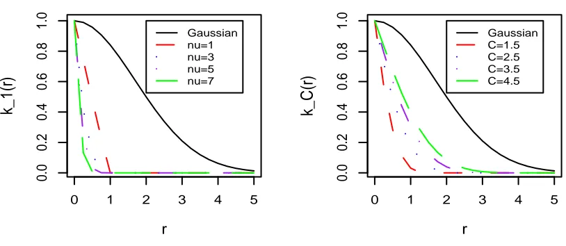
Different choices of C and ν give different compactly supported kernels. Figure 1 plots the Gaussian kernel and the derived compactly supported kernels with various values of C
andν. All the kernels are depicted as a function ofr=kx−x0k. Solid lines in both panels represent the Gaussian kernel withσ = 2.4. In the left panel,C= 1 andν varies by taking values 1,3,5,7, thus the resulting kernels have a common support [0,1]. In the right panel,
ν = 3 but C takes different values 1.5,2.5,3.5,4.5, leading to compactly supported kernels with different supports. Since ν is irrelevant to the sparsity of KC, it is generally fixed at
some value. We useν = 3 in this paper.
The following lemma shows that for a pair of inputsxandx0, the smallerC is, the more shrinkage imposed on the function value k(x,x0). This implies that the Gram matricesK
and KC can be either similar or different, depending on the choice ofC.
Lemma 1With ν fixed, for any x,x0 ∈ X,
lim
C→0 kC(x,x
0) = 0,
lim
C→∞ kC(x,x
0) = k(x,x0).
Proof: The equations are easily established by the facts: limC→0φC(kx−x0k) = 0 and
limC→∞φC(kx−x0k) = 1 for anyx,x0 ∈ X.
The use of compactly supported kernels can make predictions more efficient. For ex-ample, given the training points (x1, y1), ...,(xn, yn), the nonlinear support vector machine
(SVM) classifier trained with a kernelk is generally expressed as
f(x) =b+
n X
i=1
aik(x,xi).
To predict the label for a future observation xnew using the classifier trained with the
compactly supported kernel kC, we only need to visit those xi’s in the set δC(xnew) since f(xnew) =b+Pni=1aikC(xnew,xi) =b+Pi:xi∈δC(xnew)aikC(xnew,xi). That is, the repre-sentation of f(x) is sparse in the sense that kC(x,xi) might be zero. Trying to determine
the set δC(xnew) efficiently might be challenging though. One simple idea is to discard
all observations whose first component are not within ±C around the first component of
xnew, and compute the distance from the remaining observations toxnew, but more clever
algorithms might be constructed.
2.2 Sparse Gram Matrices
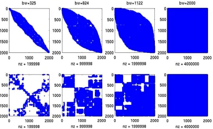
sparsity 95% 75% 50% 0 bandwidth (bw) 325 824 1,122 2,000
Table 1: Bandwidths after applying the reverse Cuthill-McKee algorithm.
Secondly, sparse matrix algorithms require much less computation time than standard algorithms by avoiding arithmetic operations on zero elements. For example, the complexity of solving a linear equation system is O(n3) for a full n×n matrix and is approximately
O(N) for a sparse matrix with certain structures. Linear systems involving sparse coefficient matrices can generally be solved very efficiently using sparse linear algebra techniques; see Gilbert et al. (1992) with an emphasis on MATLAB commands.
The entries ofKC can be reordered to have certain matrix structures convenient for
op-erations. Two commonly used techniques are reverse Cuthill-McKee algorithm (Gibbs et al. (1976), George and Liu (1981)) and the minimum degree reordering algorithm (George and Liu (1989)). The reverse Cuthill-McKee algorithm produces a matrix with a narrow band-width and generally makes nonzero elements display along the main diagonal line. For any symmetric matrix A, the bandwidth of itsith row,bi, is defined as the difference between i and the smallest column number j such that Aij 6= 0. The bandwidth of A is defined
Figure 2: Structures of KC after reordering (first row for reverse Cuthill-McKee,
by bw = 2 maxi{bi}+ 1. Bandwidth of a banded matrix is often used as a measure of its
sparsity. As an illustrative example, consider a 2,000×2,000 Gram matrix K (obtained from the green-red dataset described in Section 4) and the sparsified Gram matrix KC
with different degrees of sparsity: 95%,75%,50% and 0. Table 1 shows the bandwidth of the reordered matrix KC after applying the reverse Cuthill-McKee algorithm. The matrix
structures after reordering are plotted in the first row of Figure 2. The minimum degree procedure produces a structure with large blocks of continuous zeros, as shown in the second row of Figure 2.
3. Tuning C
It is well known that the Gram matrix contains all the information about the input data. Lemma 1 shows that the smaller C, the sparser KC is; and vice versa. Though a high
degree of sparsity is desired for computational reasons, much information may have been lost due to the sparsifying process if KC is too sparse, and the learning error may become
unacceptable. On the other hand, if KC is almost as dense as K, the efficiency gain in
computation will be limited. Therefore we need to select the thresholding parameter C
properly to balance the “information loss” and the “efficiency gain”. This is analogous to controlling the bias-variance tradeoff of estimators in statistical modeling.
3.1 Similarity and Alignment
Define the matrix ΦC by (ΦC)ij =
(1 − kxi−xjk
C )+ ν
. We will use ◦ for the Hadamard product of two matrices (element-wise product), see Horn and Johnson (1985). Then we have
KC = ΦC◦K. (2)
In order to assess the similarity between K and KC, we consider the empirical alignment
of two Gram matrices
A(C) = √ < K, KC >F
< K, K >F, < KC, KC >F
, (3)
where < K1, K2 >F=Pni,j=1K1(xi,xj)K2(xi,xj) is the Frobenius inner product between
two matrices. This alignment was first proposed in Cristianini et al. (2001) for learning kernels. It can be viewed as the Pearson correlation coefficient of two bi-dimensional vectors defined byK andKC. A convenient property ofA(C) is that it can be efficiently computed
before any training of the kernel machine takes place, only based on the input information in the training set. The following theorem shows that, for the Gram matrix KC defined in
(2), the alignment score A(C) has some nice mathematical properties as a function ofC. We take the convention 0/0 = 0 throughout this paper.
Theorem 1 Given the input set {x1, ...,xn} ⊂ X, the empirical alignment between K and KC is
A(C) =
Pn
i,j=1(ΦC)ijKij2 q
Pn i,j=1Kij2
q Pn
and has the following properties:
(i) limC→0A(C) = 0, (ii) limC→∞A(C) = 1,
(iii) A(C) is an increasing function of C.
Proof. (i) and (ii) can be easily verified using the definition ofA(C) in (3) and Lemma 1. Define rij =kxi−xjk, i, j = 1, ..., n. In order to prove (iii), it is sufficient to show that, if rij ≤C for all i, j = 1, ..., n, then
˜
A(C) =
Pn
i,j=1(1− rij
C ) νK2
ij q
Pn
i,j=1(1− rij
C )2νKij2 ,
is increasing in C. It is equivalent to show the derivative of ln[ ˜A(C)] with respect toC
D(C) = ln[ ˜A(C)]0
≥0. (4)
Since
D(C) = ν
Pn
i,j=1(1− rij
C)ν−1 rijKij2
C2
Pn
i,j=1(1− rij
C )νKij2
−ν
Pn
i,j=1(1− rij
C)2ν−1 rijKij2
C2
Pn
i,j=1(1− rij
C)2νKij2 ,
the inequality in (4) becomes
n X
i,j=1
(1−rij
C )
ν−1rijK 2 ij C2 n X i,j=1
(1−rij
C)
2νK2 ij ≥ n X i,j=1
(1−rij
C )
2ν−1rijK 2 ij C2 n X i,j=1
(1−rij
C) νK2
ij
.
(5) Define pij= 1−Crij fori, j = 1, ..., n. Then (5) is expressed as
n X
i,j=1
pνij−1(1−pij)Kij2
n X
i,j=1
p2ijνKij2
≥ n X
i,j=1
p2ijν−1(1−pij)Kij2
n X
i,j=1
pνijKij2
,
which can be further simplified to
n X
i,j=1
pνij−1Kij2 n X
i,j=1
p2ijνKij2
≥ n X
i,j=1
p2ijν−1Kij2 n X
i,j=1
pνijKij2
. (6)
Finally we can verify (6) by the following two H¨older inequalities:
n X
i,j=1
p2ijν−1Kij2 =
n X
i,j=1
p
2v2 v+1 ij K 2 v v+1 ij p
v−1 v+1
ij K 2v+11 ij ≤ n X i,j=1
p2ijvKij2v+1v n X
i,j=1
pvij−1Kij2v+11
n X
i,j=1
pνijKij2 =
n X
i,j=1
p
v(v−1) v+1
ij K
2v+1v ij p 2v v+1 ij K 2v+11 ij ≤ n X i,j=1
pvij−1Kij2v+1v n X
i,j=1
3.2 Sparsity of KC
The Gram matrixK is dense in terms of not having any zero entries. Given a training set of size n, we define the sparsity of KC relative to K by
S(C) = the number of zero entries in KC
n2 . (7)
The following theorem describes the property ofS(C) as a function ofC.
Theorem 2 Given the input set {x1, ...,xn} ⊂ X, the sparsity S(C) satisfies: (i) limC→0S(C) = 1,
(ii) limC→∞S(C) = 0,
(iii) S(C) is a decreasing function of C.
Proof. Lemma 1 implies that limC→0(KC)ij = 0 and limC→∞(KC)ij = Kij for i, j =
1, ..., n, thus (i) and (ii) hold. AsC increases, the entries ofKC become closer to those of K
and the number of zeros inKC decreases. Therefore (iii) is true by the definition ofS(C).
3.3 Similarity-Sparsity Tradeoff
For any compactly supported kernel kC, a large empirical alignment A(C) indicates little
information loss due to the sparsifying process, and a large sparsity S(C) implies a high degree of sparsity. Theorems 1 and 2 show that both A(C) and S(C) take values in the interval [0,1]; asC increases,A(C) increases butS(C) decreases. Therefore it is impossible to maximize both scores simultaneously. This similarity-sparsity tradeoff is analogous to the bias-variance tradeoff in statistical modeling to avoid overfitting. We propose three procedures to tune C adaptively, and they are all convenient to implement before any training of the kernel machine takes place.
The first procedure is to maximize a linear combination of similarity and sparsity,
maxC A(C) +γS(C). (8)
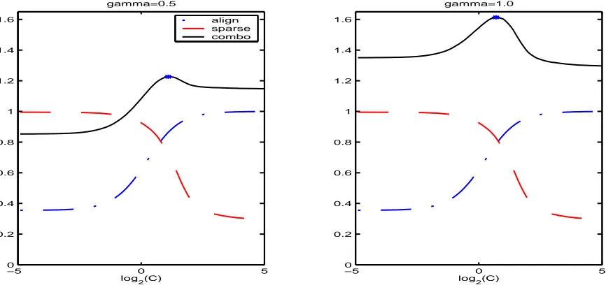
Here γ > 0 is the tuning parameter. The smaller γ is, the more weight is put on the similarity; the larger γ is, the more weight is put on the sparsity. When γ = 1, the similarity and the sparsity are equally weighted. The choice of γ depends on the nature of problems and the practical need of researchers. In Figure 3, we plot the linear combination curve with γ = 0.5 andγ = 1 in the green-red example (Example 1 in Section 4).
The second tuning procedure is to control the lower bound for information loss while maximizing the sparsity of the Gram matrix,
maxC S(C), subject to A(C)≥µ, (9)
where µ ∈ [0,1] is the desired degree of similarity. Alternatively, we can maximize the similarity A(C) conditional on a desired degree of sparsity,
−5 0 5 0
0.2 0.4 0.6 0.8 1 1.2 1.4 1.6
gamma=0.5
log 2(C)
align sparse combo
−5 0 5
0 0.2 0.4 0.6 0.8 1 1.2 1.4 1.6
log 2(C) gamma=1.0
Figure 3: Alignment (dashed-dotted lines), sparsity (dashed lines), and their linear com-bination score (solid lines) with γ = 0.5 and γ = 1. The symbol * marks the location of the optimalC where the combination score is maximized.
This third procedure is especially useful in massive dataset situations when the size of the Gram matrix is beyond computer storage limit. In practice, we can pre-evaluate the maximal number of nonzero entries that can be stored based on computer capacity, and then determine the lower bound for the degree of sparsity. For example, if only 25% of the nonzero entries in a matrix can be stored, we may choose τ = 75% and C to be the first quartile of pairwise distances {kxi−xi0k, i, i0 = 1, ..., n}.
4. Applications of Compactly Supported RBF Kernels
In this section, we illustrate the performances of compactly supported RBF kernels in three different contexts: Support Vector Machines (SVM), least squares SVM, and kernel prin-cipal component analysis. We implement all three tuning procedures proposed in Section 3.3.to select the thresholding parameter C.
4.1 Support Vector Machines
Support vector machine (SVM) is a binary classifier algorithm proposed in Boser et al. (1992), Vapnik (1995), and Vapnik (1998). Cristianini and Shawe-Taylor (2000) gave a comprehensive introduction on the SVMs. Given a training set {xi, yi}ni=1 where yi ∈
Hilbert space (RKHS) associated with the kernelk and Gram matrixK. It solves
min
b,a
1
n n X
i=1
[1−yif(xi)]++λaTKa, (11)
where f(x) =b+Pn
i=1aik(x,xi) anda = (a1, ..., an)T. The function [1−yf]+ is the
so-called hinge loss function, acting as a convex upper bound of the misclassification error. The parameter λ > 0 is a smoothing parameter. Define y = (y1, ..., yn)T, Y = diag[y1, ..., yn],
1n= (1, ...,1)T ∈Rn, andIqto be the identity matrix of sizeq×q. In general, the following
dual problem of (11) is solved with respect to the dual variables α= (α1, ..., αn)T:
maxα W(α) =−1 2(αY)
TK(
αY) +1Tnα, subject to 0≤α≤λ1n, αTy= 0. (12) This is a quadratic programming with linear constraints. With the compactly supported RBF kernel, we need to solve (12) withKreplaced byKC. Some software packages can take
advantage of the sparse structure of KC, for example the TOMLAB (http://tomlab.biz)
and the SPRNLP (http://tomlab.biz/products/sprnlp), and optimize the quadratic objective more efficiently with KC than with K. For large datasets, this efficiency gain in
computation can be very substantial.
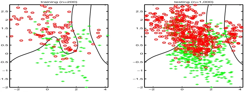
Example 1: Let us consider the green-red example used in Hastie et al. (2001). Two classes are labeled as “green” and “red”, each consisting of a mixture of ten Gaussian clusters. Ten centers mk’s of the green class are generated from the bivariate Gaussian
distributionN2((1,0)T, I2), and those of the red class are fromN2((0,1)T, I2). Figure 4 plots
the centers of two classes (large circles). For each class, 100 observations are generated as follows: for each observation, we pick anmkat random with probability 1/10 and generate
a data from an N2(mk, I2/5). To evaluate the classification accuracy of the SVM solutions,
we also generate 1,000 test data points.
−2 0 2 4
−2 −1.5 −1 −0.5 0 0.5 1 1.5 2 2.5
training (n=200)
−2 0 2 4
−2 −1.5 −1 −0.5 0 0.5 1 1.5 2 2.5
testing (n=1,000)
−5 −4 −3 −2 −1 0 1 2 3 4 5 0.2
0.3 0.4 0.5 0.6 0.7 0.8 0.9 1 1.1 1.2
log2(C)
score
Alignment A(C) and Sparsity S(C) for Example 1
alignment sparse
Figure 5: Alignment A(C) (solid line) and sparsity S(C) (dashed line) as a function ofC. The horizontal dotted lines correspond to differentµ: 0.90,0.95,0.98, and 0.99.
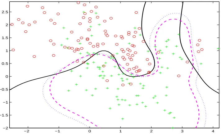
−2 −1 0 1 2 3 4
−2 −1.5 −1 −0.5 0 0.5 1 1.5 2 2.5
Figure 6: Classification boundaries given by the Bayes rule (solid line), SVM with Gaussian kernel (dotted line), and SVM with compactly supported kernel (dashed line).
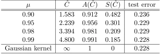
µ Cˆ A( ˆC) S( ˆC) test error 0.90 1.583 0.912 0.482 0.236 0.95 2.239 0.956 0.301 0.229 0.98 3.394 0.981 0.209 0.229 0.99 4.800 0.991 0.185 0.228
Gaussian kernel ∞ 1 0 0.228
Table 2: SVM fitting with Gaussian kernel and compactly supported kernels.
kCˆ. The smoothing parameter λin the SVM is tuned with 10-fold cross validation. Table
2 summarizes the optimal value ˆC, A( ˆC), and S( ˆC) for each choice of µ. When µ= 0.99, the SVM solution obtained with kCˆ gives the same accuracy as the solution with k, but
the Gram matrix KCˆ has the sparsity 18.5%. When µ= 0.95, though the test error of the
solution withkCˆ increases slightly from 0.228 to 0.229, the sparsity of the associated Gram
matrix increases to 30.1%. Whenµ = 0.90, the test error of the solution with kCˆ is 3.5%
higher than the solution withk (0.236 vs 0.228), but 48.2% of the entries inKCˆ are zeros.
Figure 6 plots the classification boundaries given by the Bayes rule, the SVM solution with
k, and the SVM solution withkCˆ corresponding toµ = 0.98. The Bayes rule has the test
error 0.218, which is the optimal rate using the true distribution of the data.
4.2 Least Squares Support Vector Machines
Regularized least squares classification was suggested in Poggio and Girosi (1990) and inves-tigated in Rifkin et al. (2003). Recently the least squares support vector machine (LS-SVM) was used as a variant of SVM by Suykens and Vandewalle (1999) and Suykens et al. (1999). The advantages of the LS-SVM include its good classification accuracy and easy imple-mentation by solving a linear equation system. This can make a dramatic difference in computation cost for large datasets compared to the standard SVM, where a quadratic programming has to be employed. In theory both LS-SVM and SVM target on the Bayes rule asymptotically; see Lin (2002).
The LS-SVM seeks a separating hyperplane f(x) =b+Pn
i=1aik(x,xi) by solving
min
b,a
1
n n X
i=1
1−yif(xi) 2
+λaTKa. (13)
The coefficients b anda= (a1, ..., an)T are the solution of the following linear system:
0 1Tn
1n K+1λIn b
a
=
0
y
. (14)
One standard technique for solving a linear system is the Cholesky factorization. Sparse linear systems arise by replacingK withKC in (14). The advantage of usingKC is that it
−2 −1 0 1 2 3 4
−2
−1
0
1
2
3
Standard SVM
x
y
−2 −1 0 1 2 3 4
−2
−1
0
1
2
3
Standard LS−SVM
x
y
−2 −1 0 1 2 3 4
−2
−1
0
1
2
3
LS−SVM + Compact Kernel
x
y
−2 −1 0 1 2 3 4
−2
−1
0
1
2
3
LS−SVM + Cut−off Kernel
x
y
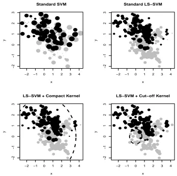
Figure 7: Bubble plots for absolute values of ai (the larger the ai the larger the bubble):
Standard SVM+RBF (top left); Standard LS-SVM +RBF (top right); LS-SVM + compactly supported RBF withν= 3 andCtuned by similarity-sparsity tradeoff (bottom left); LS-SVM + 10% cut-off RBF (bottom right).
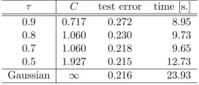
Example 2: Generate a large dataset of size n = 5,000 from the green-red example used in Example 1. We fit the least squares SVM with the standard Gaussian kernel and compactly supported kernels for which the optimal C is chosen with the third procedure in Section 3.3. We allow τ to take different values 90%,80%,70% and 50%, and the cor-responding ˆC is thus the 10th, 20th, 30th, and 50th percentile of the pairwise distances
{kxi−xi0k, i, i0 = 1, ..., n}. The smoothing parameterλis selected with an extra tuning set
of size 3,000 generated from the same distribution. Table 3 shows that the compactly sup-ported kernels may give comparable accuracy as the Gaussian kernel, but with substantial savings in computation. When τ = 0.5, the LS-SVM solution with kCˆ gives the test error
τ C test error time [s.]
0.9 0.717 0.272 8.95
0.8 1.060 0.230 9.73
0.7 1.060 0.218 9.65
0.5 1.927 0.215 12.73
Gaussian ∞ 0.216 23.93
Table 3: Least squares SVM fitting with Gaussian and compactly supported kernels.
time by 47% (12.73 vs 23.93 seconds). When τ = 0.7, the compactly supported kernel solution has the test error 21.8%, which is slightly worse than the Gaussian kernel, but saves the computation time by 60%.
To show the “local” property of the classifier given by the compactly supported kernel, we depict bubble plots for theai’s of the least square SVM solutions in Figure 7. Here the
small dataset of size n= 200 from Example 1 is used. The radius of a bubble denotes the correspondingaiin absolute value. For evaluating the function value at some examplexnew,
all the points falling outside its neighbor δC(xnew) need not to be accessed. In top panels,
all the coefficientsai’s in the SVM and LS-SVM solutions obtained with the Gaussian kernel k are different from zero. Therefore, the classification of a new input is based on all the training points. However with compactly supported kernels, only training points located in a circle (dashed curves in bottom panels) centered at xnew and of radius C are necessary.
The 10% cut-off RBF consists in defining C as the 10% percentile of the sorted set of all distances between the input points.
4.3 Kernel Principal Component Analysis
Kernel principal component analysis (Sch¨olkopf and Smola (2002)) is a kernel-based method for performing a nonlinear form of principal component analysis, and it has been an effective approach for feature extraction. Assume a nonlinear map Φ :X → H maps the data from the input space into some feature space Hassociated with the kernel k,
k(x,x0) =<Φ(x),Φ(x0)>H, (15)
where < ·,· >H is the dot product defined in H. The Gram matrix K is defined by
Kij=<Φ(xi),Φ(xj)>H. In general, the feature spaceHcontains many nonlinear features
of input variables or their high-order interactions, thus it can have a large or possibly infinite dimension. We assume the data in H is centered, that is, satisfying Pn
i=1Φ(xi) = 0, and
has the covariance matrix Σ = n1 Pn
i=1Φ(xi)Φ(xi)T. Σ is positive definite, and it has n
non-negative eigenvaluesλ1 ≥ · · · ≥λn≥0 and the corresponding normalized eigenvectors
v1,· · · ,vn. Assume only the first p λi’s are nonzero eigenvalues. Then for any point Φ(x)
the principal components are given by the p projections < Φ(x),vj >H for j = 1, ..., p.
Sch¨olkopf and Smola (2002) introduced an algorithm to perform the kernel PCA efficiently. They showed that the λi’s are also eigenvalues of 1nK, with the corresponding normalized
−1 0 1 −0.5
0 0.5 1 1.5
Eigenvalue=0.147
−1 0 1
−0.5 0 0.5 1 1.5
Eigenvalue=0.134
−1 0 1
−0.5 0 0.5 1 1.5
Eigenvalue=0.051
−1 0 1
−0.5 0 0.5 1 1.5
Eigenvalue=0.050
−1 0 1
−0.5 0 0.5 1 1.5
Eigenvalue=0.049
−1 0 1
−0.5 0 0.5 1 1.5
Eigenvalue=0.039
−1 0 1
−0.5 0 0.5 1 1.5
Eigenvalue=0.036
−1 0 1
−0.5 0 0.5 1 1.5
Eigenvalue=0.034
Figure 8: Kernel PCA using compactly supported RBF kernels.
point x, we can compute the projections onto v1, ...,vp by
<Φ(x),vj >H=
n X
i=1
αjik(xi,x), forj= 1, ..., p.
Example 3: We consider the three-cluster example in Sch¨olkopf and Smola (2002) and conduct the kernel PCA with the compactly supported kernels. Each cluster consists of 30 points generated from a bivariate Gaussian, with the center [−0.5 −0.2]T,[0 0.6]T,[0.5 0]T respectively and the common covariance matrix 0.01I2. The optimal cut-off value ˆC= 0.758
is chosen by maximizing the combinationA(C) +γS(C) withγ = 0.3, andKCˆ has the
spar-sity 0.559 and alignment 0.936. Figure 8 plots the first eight nonlinear principal components extracted using the kernel kCˆ. We observe that the first two principal components have
5. Conclusion and Discussion
We propose a method for systematically sparsifying radial basis function kernels such that the resulting kernel is compactly supported, and hence has a sparse Gram matrix. The resulting sparse property of the Gram matrix can produce crucial advantages when dealing with massive datasets in terms of demanding much less computation time and storage space. We suggest a unified framework to balance the efficiency gain and information loss due to the sparsifying operation, which provides an adaptive tuning approach for the thresholding parameter.
In theory, it is required that the power term ν > d+12 in equation (1) to ensure the positive definiteness of the sparsified Gram matrix. This condition is easy to satisfy when
d is small or moderate, but can be very restrictive for high dimensional data as in our last example whered= 256. Surprisingly, even when we use a small value ofν= 3 or 5 for such datasets, the compactly supported RBF kernel gives comparable classification performances as the traditional support vector machines while enjoying the sparsity advantage. The reason behind this observation will be investigated in the future.
For any positive definite matrix, its eigenvalues (spectrum) and eigenvectors contain much essential information about it. Some of our limited experience suggest that it is possible to describe the similarity between K and KC based on their spectrum. It is our
future work to study how this measure is related to the sparsity of KC.
Acknowledgments
We would like to acknowledge support for this project from the National Science Founda-tion grant DMS-0405913 and the Statistical and Applied Mathematical Science Institute (SAMSI) program on Data Mining and Machine Learning during 2003-2004.
References
D. Achlioptas, F. McSherry, and B. Sch¨olkopf. Sampling techniques for kernel methods.
Advances in Neural Information Processing Systems, 14:335–342, 2002.
B. E. Boser, I. M. Guyon, and V. Vapnik. A training algorithm for optimal margin classifiers.
Fifth Annual ACM Workshop on Computational Learning Theory, Pittsburgh, PA, pages 144–152, 1992.
C.J.C. Burges. Simplied support vector decision rules. In Proceeding of the 13th Interna-tional Conference on Machine Learning, Morgan Kaufmann, pages 71–77, 1996.
N. Cristianini and J. Shawe-Taylor. Introduction to Support Vector Machines. Cambridge University Press, 2000.
N. Cristianini, J. Shawe-Taylor, A. Elisseeff, and J. Kandola. On kernel target alignment.
M. S. Floater and A. Iske. Multistep scattered data interpolation using compactly supported radial basis functions. Journal of Computational and Applied Mathematics, 73:65–78, 1996.
M. G. Genton. Classes of kernels for machine learning: a statistics perspective. Journal of Machine Learning Research, 2:299–312, 2001.
A. George and J.W-H. Liu. Computer Solution of Large Sparse Positive Definite Matrices. Prentice Hall, 1981.
A. George and J.W-H. Liu. The evolution of the minimum degree algorithm.SIAM Review, 31:1–19, 1989.
N. E. Gibbs, W. G. Poole, and P. K. Stockmeyer. An algorithm for reducing the bandwidth and profile of a sparse matrix. SIAM Journal on Numerical Analysis, 13:236–250, 1976. J. R. Gilbert, C. Moler, and R. Schreiber. Sparse matrices in matlab: design and
imple-mentation. SIAM Journal on Matrix Analysis, 13(1):333–356, 1992.
T. Gneiting. Compactly supported correlation functions. Journal of Multivariate Analysis, 83:493–508, 2002.
B. Hamers, J. A. K. Suykens, and B. De Moor. Compactly supported RBF kernels for sparsifying the gram matrix in LS-SVM regression models. Proceedings ICANN, pages 720–726, 2002.
T. Hastie, R. Tibshirani, and J. Friedman. The Elements of Statistical Learning. Springer, 2001.
R. A. Horn and C. R. Johnson. Matrix Analysis. Cambridge University Press, New York, NY, 1985.
Y. Lin. SVM and the Bayes rule in classification. Data Mining and Knowledge Discovery, 6:259–275, 2002.
E. Osuna, R. Freund, and F. Girosi. An improved training algorithm for support vector machines. In J. Principe, L. Gile, N. Morgan, and E. Wilson, editors, Neural networks for signal processing VIII - Proceedings of the 1997 IEEE workshop, pages 276–285. New York, IEEE, 1997.
T. Poggio and F. Girosi. Networks for approximation and learning. Proceedings of IEEE, 78:1481–1497, 1990.
R. Rifkin, G. Yeo, and T. Poggio. Regularized Least-Squares Classification. In J.A.K. Suykens, G. Horvath, S. Basu, C. Micchelli, and J. Vandewalle, editors, Advances in Learning Theory: Methods, Models and Applications. IOS Press, Amsterdam, 2003. R. Schaback. Creating surfaces from scattered data using radial basis functions.
B. Sch¨olkopf, C. J. C. Burges, and A. J. Smola. Advances in Kernel Methods - Support Vector Learning. MIT Press, Cambridge, MA, 1999.
B. Sch¨olkopf and A. J. Smola. Learning with Kernels. MIT Press, Cambridge, MA, 2002. A. J. Smola, O. L. Mangasarian, and B. Sch¨oelkopf. Sparse kernel feature analysis. In
24th Annual Conference of Gesellschaft fr Klassifikation, University of Passau, Passau, Germany, 2000.
A. J. Smola and B. Sch¨olkopf. Sparse greedy matrix approximation for machine learn-ing. In Proceeding of the 17th International Conference on Machine Learning, Morgan Kaufmann, pages 911–918, 2000.
J.A.K. Suykens, L. Lukas, P. Van Dooren, B. De Moor, and J. Vandewalle. Least squares support vector machine classifiers: a large scale algorithm. EFFTD’99 European Conf. on Circuit Theory and Design, pages 839–842, 1999.
J.A.K. Suykens and J. Vandewalle. Least squares support vector machine classifiers. Neural Proceeding Letters, 9(3):293–300, 1999.
V. N. Vapnik. The Nature of Statistical Learning Theory. Springer, New York, 1995. V. N. Vapnik. Statistical Learning Theory. Wiley, 1998.
H. Wendland. Piecewise polynomial, positive definite and compactly supported radial basis functions of minimal degree. Advances in Computational Mathematics, 4:389–396, 1995. C. K. I. Williams and M. Seeger. Using the Nystrom method to speed up kernel machines.