Nonlinearity Tests For Bilinear Time Series Data

Jurnal Teknologi, 42(C) Jun. 2005: 1–10 © Universiti Teknologi Malaysia

1

Institut Sains Matematik, Universiti Malaya, Kuala Lumpur, Malaysia. Email: [email protected] 2

Fakulti Kejuruteraan, Universiti Kebangsaan Malaysia, 43600 UKM Bangi, Selangor, Malaysia. Email: [email protected]

3

Pusat Asasi Sains, Universiti Malaya, Kuala Lumpur, Malaysia. Email: [email protected]

NONLINEARITY TESTS FOR BILINEAR TIME SERIES DATA

IBRAHIM MOHAMED1, AZAMI ZAHARIM2, & MOHD. SAHAR YAHYA3

Abstract. This paper discusses two nonlinearity tests in time series analysis, which are the Keenan’s test and F-test. The tests are based on time domain approach and are computationally less complex than the frequency domain approach. Both tests are especially suitable for data generated from bilinear model as both can be expressed in Volterra expansion form. In this study, programs for both tests are developed in S-Plus 2000 package. Through simulation studies, it will be shown that the tests work well to distinguish linear from nonlinear data set generated from bilinear model. The nonlinearity tests were applied on four real data sets which have nonlinear characteristics and the results obtained are desirable.

Keywords: Keenan’s test, F-test, nonlinearity test, bilinear

Abstrak... Kertas kerja ini membincangkan dua ujian tak linear bagi data siri masa iaitu Ujian Keenan dan Ujian-F. Ujian-ujian ini adalah berdasarkan pendekatan domain masa dan menggunakan pengiraan yang tidak kompleks jika dibandingkan dengan pendekatan domain frekuensi. Kedua-dua ujian sangat sesuai digunakan ke atas data bilinear disebabkan keduanya boleh diungkapkan ke bentuk kembangan Volterra. Di dalam kajian ini, kami membangunkan program khas untuk ujian-ujian di dalam pakej S-Plus 2000. Kami akan menunjukkan melalui kajian simulasi bahawa ujian-ujian tersebut berfungsi dengan baik untuk membezakan data linear dan data tak linear daripada model siri masa bilinear. Ujian-ujian tak linear tersebut telah digunakan ke atas empat set data yang mengandungi ciri-ciri tak linear dan keputusan yang dihasilkan adalah baik.

Kata kunci: Ujian Keenan, Ujian-F, ujian tak linear, bilinear 1.0 INTRODUCTION

In this paper, two nonlinearity tests are used to detect nonlinearity in the time series data. Both cases are based on time domain approach and suitably applied on data generated from bilinear model.

2.0 METHODOLOGY

Before fitting a nonlinear time series model to a given set of data, it is good if the nonlinearity characteristics of the data can be detected. There are various tests that have been suggested over the past years to distinguish linear from the nonlinear data sets. For example, Subba Rao et al. [1] and Hinnich [2] used the bispectrum test. They used the fact that the squared modulus of the normalized bispectrum is constant when the time series is linear. The hypothesis is based on the non-centrality parameter, λi, which is the parameter of the σ χ λN 22 2

( )

where N is the sample size. Yuan [3] modified the Hinnich’s test in such a way that the parameter being tested under the null hypothesis is no longer λi but the location parameters, such as the mean or variance. The above mentioned methods are based on frequency domain approach.

Recently, Wu and Hung [4] proposed a detecting procedure to identify nonlinear time series data by the use of neural network. The procedure makes use of the fuzzy entropy as a measure for classification. The boundaries of the classification region are made up of the appropriate fuzzy membership functions.

On the other hand, several authors proposed time domain based nonlinearity tests. Petrucelli and Davies [5] proposed a nonlinearity test for SETAR model based on CUSUM. Chan and Tong [6] extended this test further. Meanwhile, Keenan [7] and Tsay [8] respectively considered the Keenan’s test and F-test where the model tested must be in Volterra series expansion form. In fact, bilinear model is a special case of the Volterra series expansion and thus, we will look at the last two tests in detail.

2.1 Time Series Models

The pioneering work in time series modelling is due to Wiener [9] who had produced a very general class of nonlinear model, called Volterra series expansion. It involves more than second-order theory and requires higher-order cumulant spectra. It is given by:

µ ∞ − ∞ − − ∞ − − −

=−∞ =−∞ =−∞

= +

∑

∑

∑

t i t i ij t i t j ijk t i t j t k

i i ,j i , j ,k

Y b e b e e b e e e (1)

ê

ê ê

ê

ê ê ê

ê ê

ê ê

ê

Most linear models can be expressed into Volterra expansion form which includes the autoregressive model of order p, AR(p), the moving average model of order q, MA(q), and the autoregressive moving average model of order p and q, ARMA(p,q). On the other hand, one of the nonlinear models which can be transformed into Volterra expansion form is the bilinear model. It is denoted by BL(p,q,r,s) and given by:

φ − θ − β − −

= = = =

=

∑

∑

∑∑

1 1 1 1

p q r s

t i t i j t j kl t k t l t

i j k l

Y Y e Y e e (2)

where Y t_t, =1, 2,…,nare the observed values, e_t, t = 1, 2, ..., n are the residuals based on historical data, and φi , θj and βkl are all real coefficients. The detailed bilinear theory can be found in Granger and Andersen [10].

2.2 Keenan’s Test

Keenan [7] adopted the idea of Tukey’s [11] one degree of freedom test for non-additivity to derive a time-domain statistic. The test is motivated by the similarity of Volterra expansions to polynomials, and is extremely simple, both conceptually and computationally. Assume that a time series Y_t, t = 1, 2, ..., n can be adequately approximated by a second-order Volterra expansion of the form:

µ − ∞ − −

=−∞ =−∞

= +

∑

∑

,

p

t i t i ij t i t j

i i j

Y c e c e e (3)

The approximation will be linear if the last term on the right-hand side is zero. Note that the general bilinear model given in (2) is a special case of (3). The Keenan’s test procedure is as follows:

(i) Regress Y_t on {1, Y_t–1, ..., Y_t–M}and calculate the fitted values {Y_t}, and the residuals, {ê_t}, for t = M + 1, ..., n, and the residual sum of squares,

2_.

s

< ê,ê > =

∑

(ii) RegressY_t2on {1, Y_t–1, ..., Y_t–M} and calculate the residuals, {ξt} for t = M +, ..., n.

(iii) Regress on ê = (ê_M+1, ..., ê_n) on ξ = (ξ_{Μ + 1}, ... ξ_n) and obtain η and F via 2

0

1

n

t t M

η η ξ

= +

 

= _{ }



∑

ê

ê

ê ê

ê ê

ê ê

ê ê ê ê

ê ê

(

)

2

2 2

, k

n M

F

ê ê η

η

− −

=

< > −

follows approximately F_1,n–2M–2 , where the degrees of freedom associated with <ê,ê> is (n – M) – M – 1.

Keenan’s test is based on the argument that if any of c_ijin (3) is non-zero, say c₁₂, then this nonlinearity will be distributionally reflected in the diagnostics of the fitted linear model, if the residuals of the linear model are correlated with Y_t–1Y_t–2. As in Tukey’s [11] non-additivity test, Keenan’s test uses the aggregated quantity Y_t2, the square of the fitted value of Y_t based on the fitted linear model, to obtain the quadratic terms upon which the residuals can be correlated. This idea is extremely valuable when the sample size is small because it only requires one degree of freedom.

2.3 The F-test

Tsay [8] modifies Keenan’s test by replacing the aggregated quantityY_t2by the disaggregated variables Y_t–iY_t–j, i, j = 1, ..., M, where M is as defined in Keenan’s test. The F-test procedure is as follows:

(i) Regress Y_ton {1, Y_t–1, ..., Y_t–M} and calculate the fitted values {Y_t} and the residuals, {ê_t}, for t = M + 1, ..., n. The regression model is denoted by:

t t t

Y =WΦ +e

where W_t =

(

)

(

)

(ii) Regress vector Z_t on {1, Y_t–1, ..., Y_t–M} and calculate the residuals, {XXXXX_ttttt}, for t = M + 1, ..., n. In this step, the multivariate regression model is

Z_t = W_tH + X_t, where Z_t is an 1

(

)

2 1

m= M M + dimensional vector defined by ZT_t =vech

(

)

(iii) Fit

ê_t = XXXXX_tttttβββββ + t∋ , t = M + 1, ..., n and define

(

)(

) (

)

2

=

T T T

t t t t t t

t

ê ê

m ê

∑

∑

∑

∑

X X X X

F ₍₄₎

ê

where the summation is over t from M + 1 to n. Here, F is asymptotically distributed as F_{m,n–m–M–1}.

This procedure can be reduced to Keenan’s test if one aggregates Z_twith weights determined by the least squares estimate of Y_t = W_tΦΦΦΦΦ + e_t to become scalar variable.

3.0 A COMPARATIVE STUDIES ON SIMULATED DATA

For illustrations, data is generated from several linear and bilinear models as given below:

(i) Model 1 : AR(2) –Y_t = 0.3Y_t–1 – 0.2Y_t–2+e_t (ii) Model 2 : AR(2) –Y_t = 0.4Y_t–1+ 0.1Y_t–2+e_t (iii) Model 3 : MA(2) –Y_t = 0.1e_t–1+ 0.2e_t–2+e_t

(iv) Model 4 : ARMA(2,1)–Y_t = 0.3Y_t–1 – 0.2Y_t–2+ 0.2e_t–1+e_t (v) Model 5 : BL(1,0,1,1) –Y_t = 0.1Y_t–1 – 0.01Y_t–2e_t–1+e_t

(vi) Model 6 : BL(2,0,1,1) –Y_t = 0.3Y_t–1+ 0.2Y_t–2 – 0.03Y_t–1e_t–1+e_t (vii) Model 7 : BL(2,0,1,1) –Y_t = 0.3Y_t–1+ 0.2Y_t–2 – 0.1Y_t–1e_t–1+e_t (viii) Model 8 : BL(2,0,1,1) –Y_t = 0.3Y_t–1+ 0.2Y_t–2 – 0.3Y_t–1e_t–1+e_t (ix) Model 9 : BL(2,0,1,1) –Y_t = 0.3Y_t–1+ 0.2Y_t–2 – 0.4Y_t–1e_t–1+e_t

(x) Model 10 : BL(3,0,1,1)–Y_t = 0.2Y_t–1− 0.2Y_t–2 + 0.2Y_t–3 – 0.4Y_t–1e_t–1 + e_t The first two models are AR(2) with opposite signs for Y_t–2, whereas the third model is MA(2). The fourth model is ARMA(2,1) and so far, no author has tested the F-test and Keenan’s test on data generated from this model. Models 5-10 are bilinear models. The difference between models 6-9 is in the coefficient of the bilinear term.

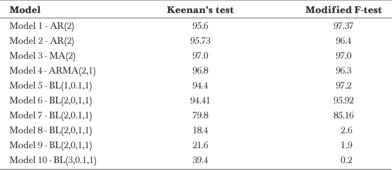
In the simulation, the e_t’s are taken to be independent N(0,1) random variate generated from rnorm object of the S-Plus [12]. For each model, generated samples are of size 200. Each sample is replicated 500 times and then tested at 0.05 significance level. The hypothesis test will be the null hypothesis of linearity against the alternative hypothesis of nonlinearity of the data. Thus, if the data is linear, with α = 0.05, more than 95% of the replicates are expected to have the test statistic less than the critical values. Summary of results is given in Table 1.

results for bilinear models do not give an outright decision of rejecting or accepting the null hypothesis of linearity since the percentages of acceptance is not less than 5%. This means that Keenan’s test may still classify nonlinear data set as linear data set. On the other hand, as the bilinear coefficients get larger, the F-test performs better as the percentages of rejection of null hypothesis become smaller than 5%. Several authors such as Chan and Tong [6] and Tsay [8] raised the same issue, saying not one nonlinearity test is enough to detect nonlinearity in a data set. Nonetheless, it is expected that the nonlinearity test will suggest whether a data set is linear or otherwise. If Keenan’s or F-test does suggest that the data is nonlinear, we expect that a bilinear model will improve the modelling of the data set. Otherwise, bilinear model may still be modelled before further inspection is carried out.

4.0 NON-LINEARITY TEST ON INDIVIDUAL SERIES

Several hydrological data sets will be used in this section to illustrate the Keenan’s test and F-test. The first set consists of the well known sunspot number series. This data set has been used as a benchmark for measuring the performance of bilinear model. Then, several local hydrological data sets will be used as further illustrations. These include the rainfall data at two weather stations in Negeri Sembilan, and water level data of two main rivers in Kelantan and Terengganu.

4.1 The Sunspot Data

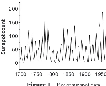
The sunspot number series, observed from 1700-1979 can be found in Box and Jenkins [13]. The series represent the number of explosion, known as sunspot, observed on the surface of the sun per year. The main feature of this series is a cycle of activity varying in duration between 9 to 14 years, with an average period of approximately

Table 1 The percentage of non-rejection of null hypothesis under the Keenan’s test and F-test

Model Keenan's test Modified F-test

Model 1 - AR(2) 95.6 97.37

Model 2 - AR(2) 95.73 96.4

Model 3 - MA(2) 97.0 97.0

Model 4 - ARMA(2,1) 96.8 96.3

Model 5 - BL(1,0.1,1) 94.4 97.2

Model 6 - BL(2,0,1,1) 94.41 95.92

Model 7 - BL(2,0.1,1) 79.8 85.16

Model 8 - BL(2,0,1,1) 18.4 2.6

Model 9 - BL(2,0,1,1) 21.6 1.9

11.3 years. It exhibits a different gradient of ‘ascensions’ and ‘descensions’, where in each cycle the rise to the maximum has a steeper gradient than the fall to the next minimum. Many authors had modelled this data using various linear and nonlinear models, such as AR(9) (see Granger and Andersen [10]), TAR(2; 3,11) (see Tong and Lim [14]), Expar(1,10) (see Subba Rao and Gabr [15]) and BL(2,1,1,1) (see Chen [16]), using various subsets of the data. Several authors such as Granger and Andersen [10], and Subba Rao and Gabr [15] had shown that bilinear model fits better on the sunspot data if compared to other linear models.

Now, the Keenan’s and F-test were used to determine whether the sunspot data is linear or nonlinear. The results are given in Table 2 where the critical values are at 0.05 level of significance. The results show that the Keenan’s test and F-test strongly support the claim that the sunspot data is a nonlinear data set.

Figure 1 Plot of sunspot data

200

150

100

50

0

Sunspot count

1700 1750 1800 1850 1900 1950

Table 2 Results of nonlinearity tests on the sunspot data

Test Test statistic Critical values Conclusion

Keenan’s test 11.02883 3.87613 Nonlinear

F-test 10.896 1.866536 Nonlinear

4.2 Local Hydrological Data

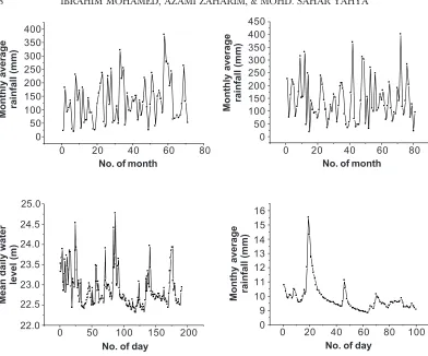
Figures 2(a) and 2(b) show the occurrence of several spikes, otherwise the plots of rainfall data are regular. On the other hand, there are a lot of spikes with high amplitudes seen in Figures 2(c) and 2(d), which is the pattern depicted by a bilinear model. Linear models may not be able to explain this characteristic adequately. Now, let us use the Keenan’s test and F-test to determine whether the data considered are linear or nonlinear. The p-values of the tests are given in Table 3.

Figure 2 Plot of several local hydrological data

400 350 300 250 200 150 100 50 0

0 20 40 60 80 No. of month

400 350 300 250 200 150 100 50 0

0 20 40 60 80 No. of month

450

Monthly average

rainfall (mm)

Monthly average

rainfall (mm)

Monthy average rainfall (mm)

16 15 14 13 12 11 10 9 0

0 20 40 60 100 No. of day

80

Mean daily water

level (m)

25.0

24.5

24.0

23.5

22.0 23.0

22.5

0 50 100 150 200 No. of day

Table 3 Results of non-linearity tests on the Sungai Lebir water level data

Data Keenan’s test F-test

Ulu Serting 0.2413 0.0000

Ladang Bahau 0.1421 0.0001

Sungai Lebir 0.0042 0.0034

For the Ulu Serting and Ladang Bahau data, the p-values of the Keenan’s test are quite large which imply that the data are linear at 10% significance level although the F-test suggests otherwise. On the other hand, both F-tests significantly identify Sungai Lebir and Sungai Kelantan data as nonlinear data due to the existence of a lot of spikes in the data.

5.0 SUMMARY

In general, the Keenan’s test and F-test are acceptably good for detecting nonlinearity for time series data generated from bilinear process, especially when the bilinear coefficient is not too close to zero. Both tests are useful to suggest whether there is any nonlinearity characteristic in the data, especially those generated from bilinear model. As shown in the nonlinear testing of Sungai Lebir and Sungai Kelantan data, data with more spikes will be identified as nonlinear data sets, which is also a characteristic of a data generated from bilinear model.

REFERENCES

[1] Subba Rao, T., and M. M. Gabr. 1980. A Test for Linearity of Stationary Time Series. Journal of Time Series Analysis. 1(1): 145-158.

[2] Hinnich, M. J. 1982. Testing for Gaussianity and Linearity of a Stationary Time Series. Journal of Time Series Analysis. 3(3): 169-176.

[3] Yuan, J. 2000. Testing Linearity for Stationary Time Series Using the Sample Interquartile Range. Journal of Time Series Analysis. 21(6): 714-722.

[4] Wu, B., and S. L. Hung. 1999. A Fuzzy Identification Procedure for Non-linear Time Series: With Example on ARCH and Bilinear Models. Fuzzy Sets and System. 108: 275-287.

[5] Petruccelli, J. D., and N. Davies. 1986. A Portmanteau Test for Self-exciting Threshold Autoregressive-type Nonlinearity in Time Series. Biometrika. 73(3): 687-694.

[6] Chan, W. S., and H. Tong. 1986. On Tests for Non-linearity in Time Series Analysis. Journal of Forecasting. 5: 217-228.

[7] Keenan, D. M. 1985. A Tukey Nonadditivity-type Test for Time Series Nonlinearity. Biometrika. 72(1): 39-44.

[8] Tsay, R. S. 1986. Nonlinearity Test for Time Series. Biometrika. 73(2): 461-466. [9] Weiner, N. 1958. Non-Linear Problems in Random Theory. Cambridge Mass: M.I.T. Press.

[10] Granger, C. W. J., and A. P. Andersen. 1978. Introduction to Bilinear Time Series Models. Gottinge: Vandenhoeck and Ruprecht.

[11] Tukey, J. W. 1949. One Degree of Freedom for Non-additivity. Biometrics. 5: 232-242. [12] S-PLUS 2000 User’s Guide. 1999. Seattle, W.A.: Mathsoft.

[13] Box, G. E. P., and G. M. Jenkins. 1976. Time Series Analysis, Forecasting and Control. San Francisco: Holden-Day.

[14] Tong, H., and K. S. Lim. 1980. Threshold Autoregression, Limit Cycles and Cyclical Data (With Discussion).

Journal of the Royal Statistical Society B. 42: 245-292.

[15] Subba Rao, T., and M. M. Gabr. 1984. An Introduction to Bispectral Analysis and Bilinear Time Series Models. Berlin: Springer-Verlag.