ABSTRACT
AZIZZADEH, SHAHRZAD. Capacity Expansion in Survivable Networks. (Under the direction of Dr.Yahya Fathi and Dr.Ranji Ranjithan.)
Capacity Expansion in Survivable Networks
by
Shahrzad Azizzadeh
A dissertation submitted to the Graduate Faculty of North Carolina State University
in partial fulfillment of the requirements for the Degree of
Doctor of Philosophy
Operations Research
Raleigh, North Carolina 2016
APPROVED BY:
Dr. John Baugh Dr. Downey Brill
Dr.Ranji Ranjithan Co-Chair of Advisory Committee
Dr.Yahya Fathi
DEDICATION
BIOGRAPHY
TABLE OF CONTENTS
List of Tables . . . vii
List of Figures . . . x
Chapter 1 Introduction . . . 1
1.1 Contributions . . . 2
1.2 Structure of the Dissertation . . . 2
1.3 Related Work . . . 3
Chapter 2 Capacity Expansion Problem in Survivable Networks . . . 5
2.1 Problem Statement . . . 5
2.1.1 Entities of the problem . . . 7
2.1.2 Statement of the problem . . . 8
2.2 Feasibility of the SNCE Problem . . . 8
2.3 Modeling Approach . . . 9
2.3.1 Origin-Destination Paths . . . 9
2.3.2 Modeling Assumptions . . . 11
2.3.3 More on Scenarios . . . 13
2.4 Model Formulation . . . 13
Chapter 3 Preparing the Model . . . 19
3.1 Finding a Set of Candidate Paths between Two Nodes . . . 19
3.1.1 Finding All Paths between Two Nodes . . . 20
3.1.2 Selection Criteria For Candidate Paths . . . 21
3.1.3 Algorithm to Find a Set of Candidate Paths . . . 25
3.2 Pre-processing . . . 26
3.2.1 Test (1) : Identifying a simple scenario . . . 27
3.2.2 Test (2) : Identifying an infeasible scenario . . . 28
3.2.3 Identifying viable scenarios . . . 28
3.2.4 Reductions and Bounds . . . 30
Chapter 4 Constructing Instances . . . 32
4.1 Distribution Model - Overview . . . 32
4.1.1 Components of the OPDN-1 . . . 33
4.1.2 Distribution Activities . . . 34
4.2 Data Entities . . . 34
4.2.1 The network . . . 35
4.2.2 Demands . . . 35
4.2.3 Expansion Options . . . 35
4.2.4 Scenarios . . . 35
Chapter 5 Solving Model IP-1 . . . 39
5.1 Experiments with Model IP-1 . . . 39
5.2 Experiments with varying number of paths . . . 40
5.3 Concluding remarks . . . 41
Chapter 6 Heuristic Methods for Obtaining Feasible Solutions and Upper Bounds . . . 43
6.1 Basic Heuristic (BH) . . . 44
6.1.1 Basic Heuristic - Finding an Expansion Plan . . . 44
6.2 Capacity Based Rounding Method (CBR) . . . 45
6.2.1 CBR - Finding an Expansion Plan . . . 47
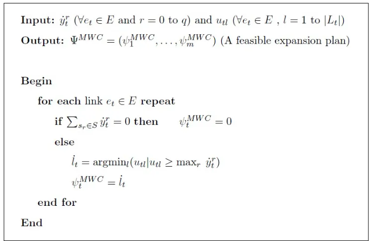
6.3 Minimum Weighted Capacity Method (MWC) . . . 49
6.3.1 MWC- Finding an Expansion Plan . . . 51
6.4 Upper Bounds and Optimality Gap . . . 52
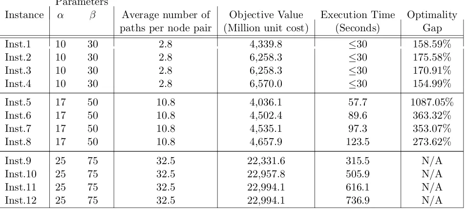
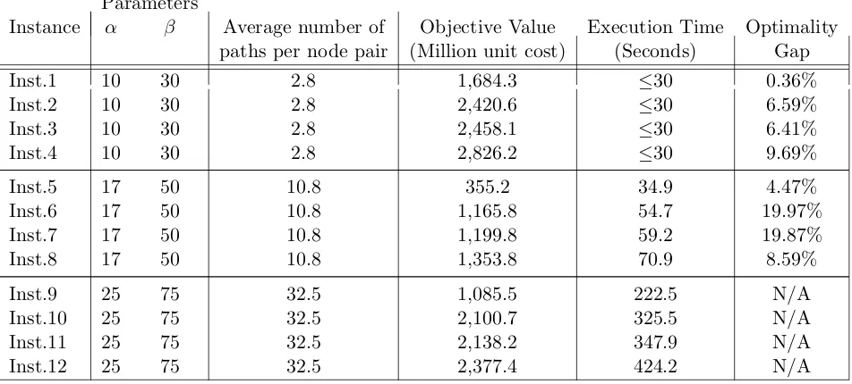
6.5 Experimental Results . . . 53
6.5.1 Summary of observations from Table 6.2 . . . 54
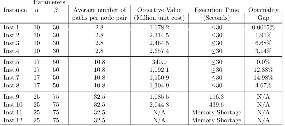
6.5.2 Summary of observations from Table 6.3 . . . 55
6.5.3 Summary of observations from Table 6.4 . . . 55
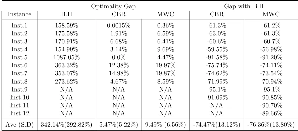
6.5.4 Summary of observations from Table 6.5 . . . 56
Chapter 7 A Delayed Constraint Generation Method for SNCE Problem . . . 58
7.1 Benders’ Decomposition Approach and Delayed Constraint Generation Algorithm 58 7.1.1 Derivation of Bender’s Decomposition Approach . . . 59
7.1.2 Delayed Constraint Generation Algorithm . . . 60
7.2 Bender’s Decomposition for Model IP-1 . . . 61
7.2.1 Implementation of the Delayed Constraint Generation Algorithm . . . 64
7.2.2 Checking the feasibility and constructing cuts . . . 65
7.3 Experimental Results . . . 66
7.3.1 Summary of Observations from Table 7.1 . . . 67
7.3.2 Summary of Observations from Table 7.2 . . . 68
7.3.3 Summary of Observations from Table 7.3 . . . 68
7.3.4 Summary of Observations from Table 7.4 . . . 69
Chapter 8 Conclusions and Future Research . . . 71
8.1 Future Research . . . 72
References. . . 74
Appendices . . . 76
Appendix A Network Data, Tables A-1 and A-2 . . . 77
Appendix B Demand Data, Tables B-1 and B-2 . . . 103
Appendix C Capacity Expansion Options Data . . . 113
Appendix D Scenarios Data . . . 114
Appendix E Optimal Expansion Plans Obtained Using a MIP Solver Directly . . . . 124
LIST OF TABLES
Table 2.1 Introductory Example : Demand . . . 11
Table 2.2 Introductory Example : Link Capacities . . . 11
Table 2.3 Introductory Example : Capacity Expansion Options . . . 12
Table 2.4 ktijf Values for the Introductory Example . . . 16
Table 2.5 Variables at the optimal solution . . . 18
Table 3.1 Links Lengths . . . 26
Table 3.2 Paths from node cto node dfor the network depicted in Figure 3.2 . . . . 26
Table 4.1 Test Instances . . . 38
Table 5.1 Execution times and optimal value at termination . . . 40
Table 5.2 Execution times and optimal value at termination for Instance 4 with varying number of paths . . . 41
Table 6.1 Capacity Expansion Options for Example 2.1 from Chapter 2, (Revisited) 45 Table 6.2 Execution times and optimal value at termination of Basic Heuristic Method . . . 54
Table 6.3 Execution times and optimal value at termination of CBR Method . . . . 55
Table 6.4 Execution times and optimal value at termination of MWC Method . . . 56
Table 6.5 Comparing the quality of the solution provided by each heuristic method . 57 Table 7.1 Number of master iterations, cuts, time and optimal value in the Delayed Constraint Generation algorithm for each instance . . . 67
Table 7.2 Comparing the execution time and optimal value obtained by solving model IP-1 directly and through Benders’ decomposition . . . 68
Table 7.3 Comparing the objective values of the solutions obtained by each method 69 Table 7.4 Comparing the optimality gap and execution times for solutions obtained by each method . . . 70
Table A.1 L1 Network . . . 77
Table A.2 L2 Network . . . 89
Table B.1 Demand Data (B1) . . . 103
Table B.2 Demand Data (B2) . . . 106
Table C.1 Capacity Expansion Options Data . . . 113
Table D.1 Scenario Data (D1) . . . 114
Table D.2 Scenario Data (D2) . . . 118
Table E.1 Optimal Expansion Plan for instance 1, obtained using a MIP solver . . . 124
Table E.2 Optimal Expansion Plan for instance 2, obtained using a MIP solver . . . 125
Table E.4 Optimal Expansion Plan for instance 4, obtained using a MIP solver . . . 126 Table E.5 Optimal Expansion Plan for instance 5, obtained using a MIP solver . . . 127 Table E.6 Optimal Expansion Plan for instance 6, obtained using a MIP solver . . . 127 Table E.7 Optimal Expansion Plan for instance 7, obtained using a MIP solver . . . 128 Table E.8 Optimal Expansion Plan for instance 8, obtained using a MIP solver . . . 129 Table F.1 Expansion Plan for instance 1, obtained by the Basic Heuristic Method . . 131 Table F.2 Expansion Plan for instance 1, obtained by the CBR Method . . . 132 Table F.3 Expansion Plan for instance 1, obtained by the MWC Method . . . 132 Table F.4 Expansion Plan for instance 2, obtained by the Basic Heuristic Method . . 133 Table F.5 Expansion Plan for instance 2, obtained by the CBR Method . . . 134 Table F.6 Expansion Plan for instance 2, obtained by the MWC Method . . . 135 Table F.7 Expansion Plan for instance 3, obtained by the Basic Heuristic Method . . 136 Table F.8 Expansion Plan for instance 3, obtained by the CBR Method . . . 137 Table F.9 Expansion Plan for instance 3, obtained by the MWC Method . . . 138 Table F.10 Expansion Plan for instance 4, obtained by the Basic Heuristic Method . . 139 Table F.11 Expansion Plan for instance 4, obtained by the CBR Method . . . 140 Table F.12 Expansion Plan for instance 4, obtained by the MWC Method . . . 141 Table F.13 Expansion Plan for instance 5, obtained by the Basic Heuristic Method . . 142 Table F.14 Expansion Plan for instance 5, obtained by the CBR Method . . . 143 Table F.15 Expansion Plan for instance 5, obtained by the MWC Method . . . 143 Table F.16 Expansion Plan for instance 6, obtained by the Basic Heuristic Method . . 143 Table F.17 Expansion Plan for instance 6, obtained by the CBR Method . . . 144 Table F.18 Expansion Plan for instance 6, obtained by the MWC Method . . . 145 Table F.19 Expansion Plan for instance 7, obtained by the Basic Heuristic Method . . 146 Table F.20 Expansion Plan for instance 7, obtained by the CBR Method . . . 147 Table F.21 Expansion Plan for instance 7, obtained by the MWC Method . . . 147 Table F.22 Expansion Plan for instance 8, obtained by the Basic Heuristic Method . . 148 Table F.23 Expansion Plan for instance 8, obtained by the CBR Method . . . 149 Table F.24 Expansion Plan for instance 8, obtained by the MWC Method . . . 150 Table F.25 Expansion Plan for instance 9, obtained by the Basic Heuristic Method . . 151 Table F.26 Expansion Plan for instance 9, obtained by the CBR Method . . . 154 Table F.27 Expansion Plan for instance 9, obtained by the MWC Method . . . 154 Table F.28 Expansion Plan for instance 10, obtained by the Basic Heuristic Method . 155 Table F.29 Expansion Plan for instance 10, obtained by the CBR Method . . . 158 Table F.30 Expansion Plan for instance 10, obtained by the MWC Method . . . 158 Table F.31 Expansion Plan for instance 11, obtained by the Basic Heuristic Method . 159 Table F.32 Expansion Plan for instance 11, obtained by the MWC Method . . . 162 Table F.33 Expansion Plan for instance 12, obtained by the Basic Heuristic Method . 163 Table F.34 Expansion Plan for instance 12, obtained by the MWC Method . . . 166 Table G.1 Expansion Plan for instance 1, obtained by the Benders’ Decomposition
Method . . . 168 Table G.2 Expansion Plan for instance 2, obtained by the Benders’ Decomposition
Table G.3 Expansion Plan for instance 3, obtained by the Benders’ Decomposition Method . . . 170 Table G.4 Expansion Plan for instance 4, obtained by the Benders’ Decomposition
Method . . . 170 Table G.5 Expansion Plan for instance 5, obtained by the Benders’ Decomposition
Method . . . 171 Table G.6 Expansion Plan for instance 6, obtained by the Benders’ Decomposition
Method . . . 172 Table G.7 Expansion Plan for instance 7, obtained by the Benders’ Decomposition
Method . . . 172 Table G.8 Expansion Plan for instance 8, obtained by the Benders’ Decomposition
Method . . . 173 Table G.9 Expansion Plan for instance 9, obtained by the Benders’ Decomposition
Method . . . 174 Table G.10 Expansion Plan for instance 10, obtained by the Benders’ Decomposition
Method . . . 175 Table G.11 Expansion Plan for instance 11, obtained by the Benders’ Decomposition
Method . . . 175 Table G.12 Expansion Plan for instance 12, obtained by the Benders’ Decomposition
LIST OF FIGURES
Figure 2.1 Introductory Example Network . . . 10
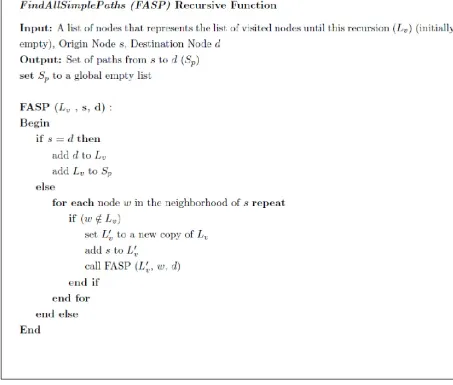
Figure 3.1 Algorithm to Find All Simple Paths between a node pair (FASP) . . . . 20
Figure 3.2 Introductory Example Network . . . 21
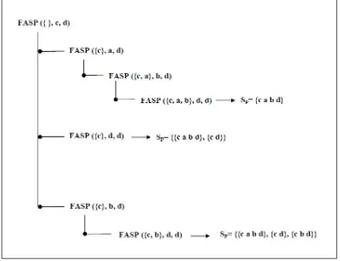
Figure 3.3 FASP function to find all paths between node c and node d for the network depicted in Figure 3.2 . . . 22
Figure 3.4 Maximum acceptable length for a path from node i to node j, as a function of the length of the shortest path from node ito node j (Lij) , with β= 10 and β = 20 . . . 23
Figure 3.5 Maximum acceptable Number of links for a path from nodeito nodej, as a function of the number of links in the Least Links path (Kij), with α = 10 andα = 20 . . . 24
Figure 3.6 Algorithm to Find Candidate Paths . . . 25
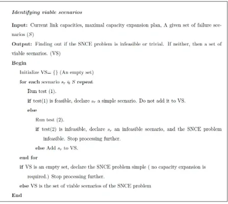
Figure 3.7 Algorithm to Identify Viable Scenarios . . . 29
Figure 4.1 Oil Products Distribution . . . 33
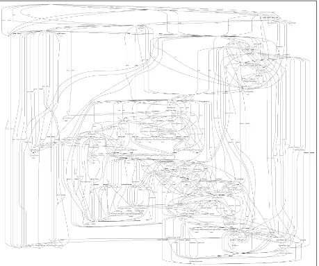
Figure 4.2 First Network (L1 Link Data Set) . . . 36
Figure 5.1 Cost of the optimal capacity expansion plan vs. number of paths included in the model . . . 42
Figure 6.1 Capacity Based Rounding Algorithm (CBR) . . . 48
Chapter 1
Introduction
Protecting critical infrastructures against possible hazardous conditions has recently been the center of attention. These infrastructures can often be represented as capacitated service net-works with specified demands that need to be satisfied. One of methods of protecting these networks is by installing additional capacities on the networks to guarantee meeting the demand under all the possible conditions the network may face. However cost-effective decision making regarding design and expansion of capacity in service network is a major challenge with signif-icant applications in telecommunication, electric power, distribution and transportation areas [1, 2, 3, 4]. In most cases cost and capacity limitations play an important role in survivable network design problems. By survivable design we mean that the multi-commodity network should be able meet all point-to-point demands under the potential failures that may happen to the network. These network capacity design (and expansion) problems are known to be NP-Hard [1].
1.1
Contributions
The contributions of this dissertation can be summarized as follows:
1. We introduce an integer programming model for the capacity design in survivable networks potentially facing many failure scenarios.
2. We implement a delayed constraint generation algorithm in the context of Benders’ De-composition, to solve instances of SNCE problem exactly within reasonable time and memory requirements.
3. We develop multiple heuristic algorithms to provide high quality and near optimal solution within reasonable time and memory requirements.
4. We describe the problem in the context of an oil products distribution network, inspired by a real-life problem. We generate multiple non-trivial instances of the problem, based on the original instance and develop pre-processing methods for the problem, including a path generation algorithm and tests for early detection of infeasibility or triviality of various scenarios, before solving the problem.
5. We presented experimental evaluation of our algorithms. Our experiments show that our proposed heuristic approaches result in high quality expansion plans and our decomposi-tion approach results in the globally optimal expansion plan.
1.2
Structure of the Dissertation
In the remainder of this chapter, we briefly review the related work. In chapter 2 we present a formal definition of capacity expansion in survivable networks and discuss the problem state-ment and concepts related to our modeling approach and assumptions. We also introduce an integer programming model (IP-1) for the SNCE (Survivable Network Capacity Expansion) problem.
In chapter 3 we discuss some model preparation techniques. These include a method on how to generate a reasonable set of paths between each origin and destination node pair in the network, to be used as an input in the optimization model. As well, tests to evaluate the feasibility and non-triviality of individual scenarios as well as the entire problem.
In chapter 5, we provide some experiments on solving model IP-1 using a commercial mixed integer programming (MIP) solver. We report our findings and make several observations on the time and memory requirements of the collection of the instances.
In chapter 6, we introduce 3 heuristic methods to provide high-quality solutions for our problem. These heuristic methods require less time and memory than the conventional MIP solver, although the resulting solutions are not guaranteed to be optimal.
All of our heuristic methods have linear programming approaches and hence they do not require a mixed integer programming solver. We provide experimental results and make several observations.
In chapter 7 we implement a delayed constraint generation method that uses a Bender’s decomposition approach to solve the SNCE problem exactly. We provide experimental results and make several observations. Finally in chapter 8 we provide conclusions of the research and also introduce a possible future direction for the research.
1.3
Related Work
Capacity design and expansion in failure prone networks is an important class of problems aris-ing in many contexts includaris-ing telecommunication, electric power and transportation networks. Extensive amount of research in this field has been done. For a few please see [4, 5, 6]. However, almost no two research work in this field has the exact same set of assumptions.
An extensive body of literature exists on capacity design in networks with uncertain demands. For a few please see [7, 8, 9] and [10]. Many branch and bound, stochastic programming, cutting plane and also approximation [11] approaches have been proposed for the problem. Riss et al [7] present a stochastic integer programming approach to the problem of network capacity expan-sion where point-to-point demand is uncertain and propose an L-shaped solution procedure to solve the problem. While our work is focused on the survivable design, (i.e., to be able to meet demands under all potential failure scenarios), many papers focus on accepting failed demands with an associated penalty [5, 6]. In the mentioned papers the main assumption is that the failure scenarios can cause link damages. Further they assume that binary damage state for links (0 or 1 as to failed or operating). A budget constraint is used to control the choice of capacity expansion option, while the objective function tries to minimize the cost associated with lost demand. They use a stochastic programming approach to the model, assuming the probability of the occurrence of each failure state is known to the decision maker.
Chapter 2
Capacity Expansion Problem in
Survivable Networks
Network capacity expansion under uncertainty is an important class of problems arising in many contexts including transportation, telecommunication and distribution networks. This problem has been the center of attention in the context of transportation and distribution networks due to increasing need for natural and man-made hazards preparedness. Civil infrastructures and service network components are usually vulnerable to large scale urban hazards such as earth-quakes, hurricanes and floods. For example the 1994 Northridge earthquake caused damage to 286 state highway bridges, out of which seven major ones collapsed [5]. A damaged trans-portation or distribution network not only affects the normal functionality of modern societies, but also directly impacts the effectiveness of post-disaster rescue and recovery activities. The importance of unimpeded operation of transportation networks raises the question of how to optimally allocate resources for installing additional capacities to the network components to improve the robustness of the entire network.
2.1
Problem Statement
Network capacity design and expansion problems are central to a large number of contexts including transportation, distribution and telecommunication. The idea is to expand a network of links (roads, pipelines, transportation means. etc.) to enable the flow of commodities (people, data, material, etc.) in order to satisfy some demand.
Applications of this class of problems can be found in many critical infrastructures that are vulnerable to large scale urban and man-made hazards, such as earthquakes, hurricanes and flood, or man-made attacks and outages. As the smooth operation of such infrastructures is important, preventive measures should be taken to minimize or avoid the possibility of service outage.
One of the preventive measures that decision makers can take to avoid the possibility of service outage or a system failure is to install additional capacities on links to guarantee sat-isfying the demand under the set of possible failure scenarios. The different failure scenarios are characterized by the availability of the links as well as demand for each scenario. The goal is that the resulting network (after capacity expansion decisions are implemented) should be resilient to failures, i.e., the network should be able to satisfy the demand under all possible failure scenarios. The decisions regarding the capacity expansions should be made with respect to the individual components and also the overall importance of the component to the perfor-mance of the whole infrastructure. This is because individual components in an infrastructure are not independent of each other. Any change in a component of the infrastructure may cause the flow of commodities to be re-distributed and therefore other components may be affected remotely. Therefore decisions should be made at the infrastructure level. The whole infras-tructure maybe modeled as a network, and the components can be represented by network links. As the decision makers are trying to protect the service provided by the infrastructure, represented by a network, against a set of possible failure scenarios, the problem is referred to as survivable network design and capacity expansion problem [12] [13] [1] and [11]. In this class of problems decision makers are mostly interested in a set of capacity expansion decisions for links that allows satisfying the demand while minimizing the cost.
Here, the node to node demands are based on the hazardous conditions the network faces and their consequences. This means that in order to have a survivable network, the decisions for capacity design and expansion cannot be based only on the demand under normal condi-tion. The amount of demand between each origin-destination node pair vary under different hazardous conditions. We call each of these conditions a failure scenario.
2.1.1 Entities of the problem 1. The Network
We assume we have a networkG= (V, E) whereV is the set of nodes andE is the set of links (with|E|=m). Associated with each link et∈E fort= 1 tom, there is an initial capacity ofut0.
There is an initial demand matrix D0 = (dij0), where the entrydij0 represents the initial demand that must be supplied from node i to node j. We assume that under normal condition the link capacities are sufficient to allow the flow of material through the network to satisfy demand for all nodes.
2. Failure Scenarios
We assume that the network described above is subject to various potential failures. The set of failure scenarios are denoted by S (with |S|= q). Individual scenarios are denote by sr ∈ S. A network failure could potentially result in a change (reduction) in the capacity of each link as well as changes in demand values. More specifically, we assume that for each scenariosr∈Sand for each linket∈E we have an associated valueλtr that represents a fraction of the capacity of linketthat remains available if failure scenariosr occurs. We further assume that for each scenariosr demand from nodeito nodej would change from dij0 todijr.
3. Expansion Options
We assume that for each linket∈E we have a set of expansion optionsLt. For each link, the options are numbered sequentially from 1 to |Lt|. Corresponding to the lth option in Lt there is a value utl that represents the increase in the capacity of link et iflth option is selected, with an associated cost ctl. We denoted the initial capacity of link et by ut0, hence if we choose to expand the capacity of link et according to the lth option, the resulting capacity will beut0+utl.
4. Decisions
The decisions in this context is to select an expansion option for each link et in the network.
5. Expansion Plan
2.1.2 Statement of the problem Given
1. A NetworkG= (V, E)
2. An initial capacity ofut0 associated with each linket 3. An initial demand matrixD0= (dij0)∀i, j∈V
4. A set of failure scenariosS with associated values ofλtr anddijr for each scenariosr∈S, and for all linkset∈E and pairs (i, j).
5. A collection of expansion options Lt for each link et ∈E with associated values utl and ctl forl= 1 to|Lt|
We seek to answer the following two questions:
1. Is there an expansion plan for the network so that it remains feasible under every failure scenario?
2. If the answer to the first question is yes, then, among all such expansion plans, find a plan that has the lowest cost.
2.2
Feasibility of the SNCE Problem
The first research question introduced above is on the feasibility of the problem. To answer this question we need to provide a definition for Maximal Capacity Expansion Plan.
Definition: Maximal Capacity Expansion Plan
If for each links et∈E the Expansion Option that provides the highest capacity is selected, the resulting Expansion Plan is called the Maximal Capacity Expansion Plan.
2.3
Modeling Approach
The proposed modeling approach is general and in principle can be used to address capacity expansion decisions in survivable networks for any type of networks, including telecommuni-cation, distribution and transportation networks. The goal of the problem is to identify the minimum cost capacity expansion plan that can satisfy the demand under every failure sce-nario. In practice, the capacity expansion decisions need to be made before any failure scenario occurs, while a second set of decisions need to be made after information about the occurrence of a failure scenario is revealed. The second set of decisions would identify how to route traffic flow on network paths based on the demand and available capacities under a failure scenario. This decision making structure suggests a framework for a two-stage decision making model, which only includes a first stage cost function (capacity expansion investments). The second stage cost is zero, implying that no cost is incurred for routing the flows in the networks once enough capacity is available. As all the demand under all failure scenarios must be met, the probability distribution of the occurrence of the scenarios is not required.
In the literature it is often assumed that links face a binary damage state (failed or undam-aged) [5], [3] and [6]; however our proposed modeling approach provides the opportunity for modeling partial failures (capacity loss) in any combination of links.
Capacity expansion decision for each link is represented by a set of binary variables with 1 representing that the expansion plan is chosen for the link and 0 otherwise. The use of binary variables for capacity expansion decisions is because in most applications it is required that links are of a modular capacity or there are only specific technological options available to be installed on each link , and having any continuous value for links capacities is simply infeasible. Rather, there are limited number of technological options available to be installed for each link which, in turn, leads to a set of distinct choices Ltfor each link t.
2.3.1 Origin-Destination Paths
Figure 2.1: Introductory Example Network
reason for every pair of nodes (i, j), if the total number of feasible paths from i to j is too large, we limit the choice of paths from nodeito nodej to a limited subset of all feasible paths between these two nodes. We denote this subset by Pij and we denote the fth path in this subset by pijf , forf = 1 to |Pij|.
For notational convenience we further define a set of binary constants over the set of links and paths. These constants provide a mapping between the links and the paths. i.e., they are used to identify which links belong to which path. We denote these binary constants by kijft , wherektijf=1 if link et belongs to path pijf and kijft =0 otherwise.
Later we describe how to determine the subset of paths Pij for every pair of nodes (i, j) with positive demand.
Example 1 To motivate the problem, we start with a simple example. Consider the network in Figure 2.1 with nodes V ={a, b, c, d} and links E={e1, e2, e3, e4, e5}. Suppose at any time the network is in either one of these two conditions: the normal condition (s0) under which the node to node demand and link capacities are at their normal level; and a failed scenario (s1) under which the demand and available capacities of links vary from normal. Under the normal condition (s0) there is a demand of 4 units between nodesa(origin) andb(destination). There is also a demand of 3 units between nodesc (origin) and d(destination). Tables A and A represent the network data under the two scenarios.
Table 2.1: Introductory Example : Demand
Demand Scenarios0 Scenarios1 Pij
dab 4 2 {pab1= (e1)}
dcd 3 4.5 {pcd1= (e3), pcd2= (e5, e1, e2), pcd3 = (e4, e2)}
Table 2.2: Introductory Example : Link Capacities Link Capacity under Scenarios0
(Normal Condition)
Capacity Coefficient under Scenarios1 (λt1)
Capacity under Scenario s1
e1 4 .25 1(=4*.25)
e2 3 1 3(=3*1)
e3 2 .5 1(=2*.5)
e4 5 .8 4(=5*.8)
e5 2 1 2(=2*1)
capacities. For example, from the data provided in Tables 2.1 and 2.2 , under failure scenario s1, the capacity of link e1 drops to 1(= 4∗0.25), whereas the demand between a and b is 2. Since pab1 = (e1) is the only path between a and b and its capacity is less than the demand (1<2), the network will not be able to meet the demand. Therefore links capacities must be expanded for the network to be able to meet the demand.
There is a set of capacity expansion options for each link, from which at most one option can be installed on each link, creating a set of mutually exclusive investment decisions for each link. The data regarding these capacity expansion options and their associated costs are presented in Table 2.3. The initial capacity of link etis shown by ut0 and the capacity of the lth expansion option for link et is shown byut1. Note that for simplicity we have assumed that each link has the same number (two) of capacity expansion options. The maximal capacity expansion plan for this network is Ψmax=(2,2,2,2,2) with the capacity expansion of (5,5,5,5,5). The network is feasible for every scenario using the maximal capacity expansion plan.
2.3.2 Modeling Assumptions
Table 2.3: Introductory Example : Capacity Expansion Options
Initial Option 1 Option 2
Link Capacity (ut0) Capacity(ut0+ut1) Cost Capacity(ut0+ut2) Cost
e1 4 4+3 10 4+5 15
e2 3 3+3 8 3+5 9
e3 2 2+3 5 2+5 7
e4 5 5+3 8 5+5 17
e5 2 2+3 2 2+5 3
combination of links and/or change in a combination of node-to-node demand. Therefore we do not assume that only one link can fail at a time, although this is a common practice in some of the previous works including [5, 2].
Followings are some key assumptions that we made ealier in defining the problem and we repeat them here for convenience.
Assumption 1 Let the random variable representing the occurrence of failure scenarios be ξ. The set of realizations of ξ is finite, i.e., it has a predetermined number of possible values ξ ∈
ξ1, ξ2, ..., ξq , where |S|=q. The possible realizations of ξ correspond to the occurrence of failure scenarioss1, s2, ..., sq, respectively.
Assumption 2 Associated with each failure scenariosr there is an array of links availability coefficients Λr=(λ1r, λ2r, ..., λmr). Eachλtr determines a fraction of capacity of link et that is available under failure scenariosr. Let the initial plus the expanded capacity of linket under the normal conditions beut0+utl ; based on this assumption, the available capacity of linket undersr would beλtr∗(ut0+ut1).
Assumption 3 Each failure scenario sr has an impact on node to node demands in the network. The demand under normal condition and under failure scenario sr are denoted by dij0 and dijr, respectively. Value ofdijr maybe larger than, smaller than, or equal to dij0.
Assumption 5 Capacity expansion decisions are mutually exclusive. Only one expansion option can be chosen for each link.
Assumption 6 Flows are routed through simple paths in the network. A simple path is a sequenced set of links that connects an origin to a destination and contains no cycle. Throughout this thesis, wherever we use the term “path” we are referring to a simple path.
2.3.3 More on Scenarios
When studying the effects of failure scenarios on links availability, from problem data, we have 0 ≤λtr ≤1 for all et ∈E. So the links availability will either remain the same, or decreases. No failure scenario results in increase of the availability of the links.
For easier reference, in all instances of SNCE problems0 is used to represent the normal condi-tion. ThereforeΛ0=(λ10, . . . , λm0)=(1,1,. . . ,1) for all instances. On the other hand, under each failure scenario the demand between each pair of nodes (i, j) could either increase (dijr> dij0), decrease (dijr< dij0) or remain the same (dijr=dij0).
Example 1 (Continued)
Given the data in Table A, we have Λ1=(0.25,1,0.5,0.8,1). Also the demand values have changed from (dab0, dcd0)=(4,3) to (dab1, dcd1)=(2,4.5).
2.4
Model Formulation
In this section we propose an integer programming model for our survivable network capacity expansion problem. We define the following notations:
Sets
V: Set of Nodes in the network, with|V|=n E : Set of Links in the network, with |E|=m
Lt : Set of Capacity Expansion Options for link et∈E S : Set of Failure Scenarios, with |S|=q
Pij : Set of Candidate Paths between node iand nodej
Data
utl : Additional capacity on link et if the lth capacity expansion option from the Lt set is installed
ctl : Cost; if the lth capacity expansion option inLtis installed on linket λtr : Coefficient of capacity of link et under failure scenariosr∈S dijr : Demand betweeniand j under scenariosr
Constant
ktijf : Binary constant, 1 if linket belongs to path pijf ; 0 otherwise
Decision Variables
ztl : Binary variable, 1 if thelth capacity expansion option in Lt is installed on linket∈E ; 0 otherwise , for all t= 1 to |E|and for alll= 1 to |Lt|
xrijf : Flow passing through path pijf under failure scenario sr , for all i, j∈V :dij0 >0 and forf = 1 to |Pij|and for all sr ∈S
Formulation of Survivable Network Capacity Expansion (SNCE)-Model IP-1
M in m
X
t=1 |Lt|
X
l=1
ctl ztl (2.1)
subject to.
|Lt|
X
l=1
ztl ≤1 t= 1 to m (2.2)
X
∀i,j∈V:dij>0
|Pij|
X
f=1
ktijfxrijf ≤λtr
ut0+
|Lt|
X
l=1 utlztl
t= 1 to m r = 0 to q (2.3)
|Pij|
X
f=1
xrijf ≥dijr ∀{i, j∈V :dij0>0} r = 0 to q (2.4)
Objective
The objective function in 2.1 is to minimize the total cost of capacity expansion decisions. The objective function only include ztl variables. This implies that as mentioned in Assumption 4 the only cost element in the problem is the cost of capacity expansion.
Mutual Exclusion Constraints
The set of constraints in 2.2 restrict the choice of capacity expansion plans to no more than one plan for each link (Assumption 5). As these inequalities represent the mutual exclusion of the capacity expansion decisions for each link, they are referred to as Mutual Exclusion Constraints.
Link Capacity Constraints
The second set of constraints (2.3) are Link Capacity Constraints. The total amount of flow passing through each link (P
∀i,j∈V:dij>0
P|Pij|
f=1kijft xrijf) should be less than or equal to the link’s available capacityλtr
ut0+P |Lt|
l=1utlztl
, for all links, under all failure scenarios.
Demand Constraints
The third set of constraints (2.4) are Demand Constraints. The total amount of flow passing through the paths betweeniandj (P|Pij|
f=1xrijf) should be greater than or equal to the demand betweeniand j (dijr), under all failure scenarios.
Example 1 (Continued)
Here, we re-visit our introductory example and formally model the problem using the modeling approach and notations introduced in the previous section. Using the data provided in Table A, we first need to determine the value of kijft .
Linke1belongs to pathspab1andpcd2, thereforekab11 =kcd21 = 1. This implies that when writing the Capacity Constraints for link e1, only the flow variables of paths pab1 andpcd2 will appear in the constraints. With the same analogy, the values of ktijf are determined and represented in Table 2.4.
Based on the data provided for Example 1 in Tables A to 2.4 , the capacity expansion problem for the network to be survivable would be as follows:
Table 2.4: kijft Values for the Introductory Example
Paths
Link pab1 pcd1 pcd2 pcd3
e1 1 0 1 0
e2 0 0 1 1
e3 0 1 0 0
e4 0 0 0 1
e5 0 0 1 0
subject to.
M utual Exclusion:
z11+z12≤1 z21+z22≤1 z31+z32≤1 z41+z42≤1 z51+z52≤1
Link e1 Capacity :
x0ab1+x0cd2 ≤4 + 3z11+ 5z12 unders0 x1ab1+x1cd2 ≤0.25 (4 + 3z11+ 5z12) unders1
Link e2 Capacity :
x0cd2+x0cd3 ≤3 + 3z21+ 5z22 unders0 x1cd2+x1cd3 ≤3 + 3z21+ 5z22 unders1
Link e3 Capacity :
x0cd1≤2 + 3z31+ 5z32 under s0 x1cd1≤0.5 (2 + 3z31+ 5z32) under s1
Link e4 Capacity :
Link e5 Capacity :
x0cd2≤2 + 3z51+ 5z52 under s0 x1cd2≤2 + 3z51+ 5z52 under s1
Demand dab :
x0ab1≥4 under s0 x1ab1≥2 under s1
Demand dcd :
x0cd1+x0cd2+x0cd3 ≥3 unders0 x1cd1+x1cd2+x1cd3 ≥4.5 under s1
zel∈ {0,1} e= 1,2, ..,5; l= 1,2 x0ab1, x1ab1, x0cd1, x1cd1, x0cd2, x1cd2, x0cd3, x1cd3≥0
The introductory example can be solved to optimality, with the optimal objective of 23. The optimal values of the capacity expansion decision variables and the flow variables are presented in Table 2.5. The results show that at the optimal solution the capacity of linke1is expanded by installing the second option (an addition of 5 units to its original capacity) and the capacity of linke2 is expanded by installing the first option (an addition of 3 units to its original capacity). The rest of the links do not need capacity expansion for the system to be survivable. So the optimal expansion plan for this example would be Ψ∗ = (2,1,0,0,0).
Table 2.5: Variables at the optimal solution ztl l=1 l=2
t= 1 0 1
t= 2 1 0
t= 3 0 0
t= 4 0 0
t= 5 0 0
Chapter 3
Preparing the Model
In this chapter we introduce preliminary concepts regarding preparing and pre-processing the model for Survivable Network Capacity Expansion (SNCE) problem. We start by discussing an algorithm to find a set of candidate paths between any origin-destination node pair in a directed network. As described in Chapter 2 Assumption 6, finding a set of candidate paths is the first step in modeling the optimization problem. Then in the following section we introduce a few tests and pre-processing methods to clean up the data and also identify possible infeasibility of the problem.
3.1
Finding a Set of Candidate Paths between Two Nodes
Given a network G=(V,E), the total number of paths between any pair of nodes can be quite large. Consequently, the number of flow variables (xrijf) in our model would also be quite large. This would result in a very large and potentially hard to solve optimization model. In practice, it is reasonable to expect the flows to be routed through “better” i.e., shorter and less costly paths [4]. For this reason, in our optimization model, for each pair of origin destination nodes i and j, we use a limited number of paths that are deemed to be more promising. However, such a set of candidate paths for those nodes does not guarantee that the set contains the optimal paths for the original problem. In many applications, however, it can be shown that this approach results in obtaining either optimal, or near optimal solutions while reducing the corresponding computational requirements to manageable levels.[14]
Figure 3.1: Algorithm to Find All Simple Paths between a node pair (FASP)
Definition: Simple Path
A simple path is a sequenced set of links that connects an origin to a destination and contains no cycle. Throughout this thesis, wherever we use the term “path” we are referring to a simple path.
3.1.1 Finding All Paths between Two Nodes
The problem of finding all paths between two nodes in a network is an NP-Hard problem. [15]. Here, we implement an adoption of a recursive algorithm presented in [15] by Thorelli. The algorithm is depicted in Figure 3.1 and is denoted by “FASP”.
Figure 3.2: Introductory Example Network
the origin node (s), the adjacent nodes are visited in a depth-first order. If the recently visited node ( denoted by w) is the same as the destination (d), then a new path is found, and that branch is fathomed. Otherwise, the recently visited node (w) is marked visited, and is then treated as the new origin node. From Figure 3.2 and Example 3.1 below, the recursive nature of the algorithm and its steps could be seen more clearly.
Example 3.1 To find all the simple paths between node pair (c, d) in the network depicted in Figure 3.2, we use the FASP algorithm. In Figure 3.3 we have shown how this recursive algorithm unfolds and results in finding all the paths between node c and node d. The first path connects the nodes in the following order: Sp={c a b d}. After the second and third paths are added, the completed set of paths would be{{c a b d},{c d},{c b d}}.
3.1.2 Selection Criteria For Candidate Paths
As mentioned earlier, instead of using all the paths between each origin destination node pair, we use a set of candidate paths. To create a set of candidate paths, we have used the following two selection criteria:
Selection Criteria 1: Length of each path
Figure 3.4: Maximum acceptable length for a path from nodeito nodej, as a function of the length of the shortest path from nodeito node j (Lij) , with β= 10 and β = 20
Selection Criteria 2: Number of links traversed in each path
In practice, often paths that traverse a limited number of links are more desirable as compared to the paths traversing too many links. Therefore we select the paths that traverse fewer links to be included in the candidate paths.
To apply the mentioned criteria, the following strategies are implemented:
Strategy 1: Limiting the length of each path
We define a parameter,M XLij, to represent the maximum acceptable length for a path from i toj. Here, we consider the shortest path to be the most efficient path between each origin-destination pair, length-wise. Therefore we try to stay within a specific gap from the length of the shortest path. Let us represent the length of shortest path from i toj by Lij. Naturally, M XLij should always be greater than or equal toLij. We also likeM XLij to have some other characteristics. We likeM XLij to always be slightly larger thanLij, to allow “good” paths in. For larger values of Lij (when the shortest path between a node pair is rather long), we like M XLij to be closer toLij, so in our candidate set, we would not be including path that are too long. We have defined the following logarithmic function that exhibits these desired behavior:
M XLij =Lij +β∗log10(Lij)
In this equation β is a coefficient determined by the user. Increase or decrease in β would allow more or fewer paths to be included in the set of candidate paths.
Figure 3.5: Maximum acceptable Number of links for a path from node i to node j, as a function of the number of links in the Least Links path (Kij), withα = 10 andα = 20
in the subsequent chapters we usedβ = 10 as the initial value. We will specify the exact value of β for each instance in Chapter 4.
Strategy 2: Limiting the number of links in each path
We define a parameter, M XHij, to represent the maximum acceptable number of links to traverse in a path fromitoj. Suppose among all the paths fromitoj, the path named “Least Links” path has the least number of links in it. To determine a reasonable value for M XHij we try to stay within a specific gap from the number of the links traversed in the the Least Links path. Let us represent the number of links in the Least Links path from ito j by Kij. Naturally, M XHij should always be greater than or equal to Kij. We also like M XHij to have some other characteristics. We likeM XHij to always be slightly larger thanKij, to allow “good” paths in. For larger values of Kij (when the Least Links path between a node pair has rather too many links), we like M XHij to be closer to Kij, so in our candidate set, we would not be including path that include traversing too many links. We also like M XHij to be an integer value, since it will be representing the maximum acceptable number of links to traverse. We have defined the following logarithmic function that exhibits these desired behavior:
M XHij =dKij +α∗
Ln(Kij + 1) Kij
e
In this equation α is a coefficient determined by the user. Increase or decrease inα would allow more or fewer paths to be included in the set of candidate paths. The ceiling function is used to assure the result is an integer value.
Figure 3.6: Algorithm to Find Candidate Paths
in the subsequent chapters we used α= 10 as an initial value. We will specify the exact value of α for each instance in Chapter 4.
3.1.3 Algorithm to Find a Set of Candidate Paths
FASP algorithm returns a sequence of nodes for each path fromitoj. We transform this form of output into a sequence of links.(When there are more than one links available between a node pair, a separate path is created to include each link.)
Table 3.1: Links Lengths Link Length
e1 10
e2 1
e3 1
e4 1
e5 10
Table 3.2: Paths from node c to nodedfor the network depicted in Figure 3.2 Path (sequence of nodes) Path (sequence of links) Length Number of Links
cd {e3} 1 1
cbd {e4, e2} 2 2
cabd {e5, e1, e2} 21 3
Example 3.2 Suppose we like to choose a set of candidate paths from node c to node din the network from the previous example (Example 3.1). The length of the links are as shown in Table A. From Example 3.1 we have the set of all paths as{{c a b d},{c d},{c b d}}.
These paths are transformed into sequences of the links. The paths before and after being transformed, along with their lengths and the number of links in them are presented in Table A. {e3}is the shortest and also the Least Links path, with Lij=1 andKij = 1. From Strategy 1 and Strategy 2 we haveM XLij=1 (with β = 10) and M XHij=4 (with α = 10). Therefore only {e3} is included in the set of candidate paths and {e4, e2} and {e5, e1, e2} are out due to their length. SoPcd={{e3}}.
3.2
Pre-processing
Given the data set for an instance of the SNCE problem, we carry out a few simple tests to clean up the data and prepare it for constructing the model. In this section we describe these tests.
A Simple Scenario
(i.e, meet all the demands under this scenario) if no expansion is made.
An infeasible Scenario
A given scenario is said to be an infeasible scenario if the network cannot accommodate this scenario (i.e, meet all the demands under this scenario) even if maximal capacity expansion plan is installed. ( All links are expanded using the option with the maximum capacity).
A Viable Scenario
A scenario is said to be a viable scenario if it is neither a simple scenario nor an infeasible scenario.
3.2.1 Test (1) : Identifying a simple scenario
To test if the network is able to meet the demands for a given scenario, given the current ca-pacities (condition (1)), the following network flow problem should be solved. It is a feasibility test with no objective function.
Test (1) for scenario Sr
M in 0
subject to.
X
∀i,j∈V:dij>0
|Pij|
X
f=1
ktijfxrijf ≤λtrut0 t= 1 to m
|Pij|
X
f=1
xrijf ≥dijr ∀{i, j ∈V :dij0 >0}
xrijf ≥0 ∀{i, j∈V :dij0 >0} f = 1. . .|Pij|
3.2.2 Test (2) : Identifying an infeasible scenario
To test if the network is able to meet the demands with maximal capacity expansion plan, (condition (2)), the following network flow problem should be solved. It is a feasibility test with no objective.
Test (2) for scenario Sr
M in 0
subject to.
X
∀i,j∈V:dij>0
|Pij|
X
f=1
ktijfxrijf ≤λtr(ut0+utˆl) t= 1 to m
|Pij|
X
f=1
xrijf ≥dijr ∀{i, j ∈V :dij0 >0}
xrijf ≥0 ∀{i, j∈V :dij0 >0} f = 1. . .|Pij|
In this problem utˆl is the additional capacity on link et if the maximal capacity expansion plan is installed. If this problem is infeasible, then the test fails. Because then it can be concluded that for this scenario, the network will not be able to meet the demands even with the maximal expansion plan. Therefore, this scenario is infeasible to satisfy in the context of our problem. If there exists an infeasible scenario in the given set of the scenarios, we can immediately answer the first research question introduced in Chapter 2: There is no expansion plan so that the network remains feasible under every given failure scenario.
3.2.3 Identifying viable scenarios
3.2.4 Reductions and Bounds
In this section we first introduce a few simple methods that may help reduce the size of the problem. They will also simplify referring to the expansion plans and failure scenarios later when providing solution approaches. After these methods are applied, it will be easier to organize the problem’s data.
Note 1 For two possible capacity expansion options ¯l and ˆl for link et, If ct¯l > ctˆl and ut¯l≤utˆl, then the option¯lis dominated by the optionˆland¯lcan be removed from the collection
of expansion options for this link .
This mathematically trivial note states that if among the available capacity expansion op-tions for a link, one is suggesting more cost and less (or equal) capacity, then it is redundant and can safely be removed from the problem during pre-processing. After removing any possible capacity expansion options that has the condition stated in Note 1, the indices of the remaining options will be reordered such that utl ≤ utl+1 and ctl ≤ ctl+1 , l = 1. . .|Lt|,∀et ∈ E , to reference the expansion options and variables of the problem more easily.
Suppose the results of this note is applied. If by using the Maximal Capacity Expansion Plan the problem is feasible, then we will also get a trivial upper bound on the objective func-tion, which is equal to the sum of the costs of the costliest expansion options for each link.
Example 3.3
Recall the network in Example 1 from Chapter 2. From Table G the cost of the Maximal Capacity Expansion Plan will be computed as (15+9+7+17+3)=51, which is an upper bound on the optimal objective of the problem, 23, as computed in Chapter 2.
Note 2 If there exist two failure scenarios s¯r and sˆr such that λt¯r≤λtˆr ∀et∈E
and
dij¯r≥dijrˆ ∀{i, j ∈V :dij0>0}
then the Link Capacity and Demand constraints representing failure scenario sˆr will be
redun-dant and can be removed from the model without affecting the feasible region and the optimal solution.
feasible under sr¯, will also be feasible under srˆ, therefore the constraints representing sˆr are redundant.
Lower Bounds on the Objective Function:
Chapter 4
Constructing Instances
In this chapter we construct the data set for several instances of the survivable network capac-ity expansion (SNCE) problem. In the next chapter we use these instances in a computational experiment to evaluate the effectiveness of the integer programming model that we proposed for solving this problem. Subsequently in the following chapters we propose alternative method-ologies for solving this problem and employ the same instances to evaluate the effectiveness of the methodologies.
The instances we construct here are based on an oil products distribution network, inspired by a real world case. Due to the critical role of oil products in the economy as well as people’s day to day needs, this network needs to be survivable. We start by providing an overview of the problem in the context of this Oil Products Distribution Network (OPDN-1) and will then discuss data entities of the problem. We continue the chapter by providing details on how we have constructed additional instances of the SNCE problem.
4.1
Distribution Model - Overview
OPDN-1 is a network responsible for daily distribution of over 230 million litres of oil products. The network consists of 230 consumption regions, 86 oil products warehouses, and several refineries and import/export points that together form the distribution model.
Figure 4.1: Oil Products Distribution
4.1.1 Components of the OPDN-1
Products
The products distributed through OPDN-1 are Gasoline, Kerosene, Diesel fuel and Fuel oil.
Refineries
Refineries provide the products mentioned above to meet the demands. Each refinery has a large depot, where the refined products are kept temporarily before being sent to warehouse, via pipelines and railroad tanks.
Warehouses
There are 86 local warehouses (including airport fuel depots) in the OPDN-1. They receive the oil products from the refineries, store and finally sell and distribute them to various consumers and retailers, including power plants and gas stations. There are 230 consumption regions in the distribution model, each has been assigned to one or more warehouses.
Means of Transportation
(the need for pumping stations, product flow sequencing and the speed of 3-8 miles per hour), they are the most economical mean for transporting oil products for large quantities over long distances.
4.1.2 Distribution Activities
In OPDN-1, the products are delivered from refineries and import points to warehouses and export points. Therefore, in addition to the direct supply of products from refineries to ware-houses, import, export and other distribution activities are also involved in the model. Here we will introduce these activities briefly.
Import
Two major products (Gasoline and Diesel Fuel) are imported and then transported from the import points to the warehouses.There are 13 import points in OPDN-1.
Export and Bunkering
Some limited amount of oil products are transported from the refineries to export points. There are 5 export points in OPDN-1.
Bunkering is the process of supplying ships with fuel, for their own use. The product sold during this process is Fuel oil. Bunkering occurs at the same points as export occurs, and it goes under the category of export activities.
Swap
Swapping oil products is the process of receiving products at an import point and delivering it to an export point. There are several strategic reasons for this process.The product transported during the process of swapping in this network is Fuel oil. Swapping occurs at the same points were import and export occurs and it goes under the category of import and export activities. This process creates an input into the import points and increases demand at the export points.
4.2
Data Entities
4.2.1 The network
The network is given as a data set containing the links that connect the nodes of the oil products distribution network (refineries, warehouses and import and export points) to each other. In this study we consider two distinct link data sets (L1 and L2), compromising 2 networks. L1 is the original network and we have constructed L2 by adding some links to the original network. The structure of the first network is depicted in Figure 4.2. The links data set representing the first and second networks are provided in Appendix A, Tables A-1 and A-2. Each row of these tables represents a link on the network and identifies its origin, destination, length (in Kilometer) and initial capacity (in Million Liters per year). The initial capacity of each link is the sum of the capacities of the transportation means on that link. For example if two nodes are connected via a pipeline and a railroad, their connection is represented via a single link with the capacity equal to the sum of the capacities of the pipeline and the railroad.
4.2.2 Demands
As mentioned in Chapter 2, there is an initial demand matrixD0 = (dij0), wheredij0represents the initial demand that must be supplied from nodeito nodej. In this study we consider two distinct demand matrices (B1 and B2). The data sets representing these demands are provided in Appendix B, Tables B-1 and B-2, respectively. Each row in these tables represents a specific demand valuedij0 and identifies its origin, destination and its value in Million Liters.
4.2.3 Expansion Options
As discussed in Chapter 2, we assume that for each link et ∈ E we have a set of expansion options Lt to select from. In OPDN-1, the same set of expansion options are available to all the links. The data set called C1, representing these expansion options is provided in Appendix C. Each row in this table represents an expansion option along with its associated capacity (in Million Litres per Year) and cost (in unit cost per Kilometer). The cost of the expansion option for each link is then calculated as the length of the link in Kilometer (from Appendix A-1) times the cost per Kilometer. For example for link (Aril,Khhal) ( Link no.1 in Appendix A-1) the cost of installing the option ‘Pipe04‘ would be (111 Km)*(111,847 Unit cost/Km)=12,415,017 unit cost.
4.2.4 Scenarios
asR1,R2,R3 and R4. The scenarios in collection R1 are displayed in Appendix D, Tables D-1 and D-2. This collection consists of 100 scenarios. In Table D-1, each row of the table specifies the scenario identification number (r inSr), the origin and destination of each linketinvolved in that scenario and the link availability coefficient λtr. In Table D-2, each row of the table specifies the scenario identification number (r inSr), the origin and destination of each demand dijr involved in that scenario and the ratio dijr/dij0. dijr value is then calculated using this ratio and the value of dij0 from Tables B-1 or B-2, in Appendix B. Each and every scenario given in these tables is a viable scenario (i.e., is neither a simple scenario nor an infeasible scenario). CollectionsR2,R3 andR4 consist of the first 85 scenarios, the first 79 scenarios and the first 51 scenarios in R1, respectively. It is worth mentioning that the links and demands involved in the set of scenarios are selected from L1 link set and D1 demand set, so the links and demands that are involved in the scenarios are available on all the instances listed in Table 4.1.
4.3
Constructing Instance
Given the two networks L1 and L2 , two demands data sets B1 and B2, the four collections of scenarios R1 through R4 and the set of expansion options C1, we have constructed 12 instances of the problem, in 3 groups. In each group instances have the same network structure, demands and expansion options, and we only vary the failure scenarios of the network. These instances are described in Table 4.1. This set of instances will be used through the rest of the dissertation to evaluate different solution approaches and algorithms.
Table 4.1: Test Instances
Instance Network Demand Set Scenario Collection Expansion Options Set
Instance 1 L1 D1 R4 C1
Instance 2 L1 D1 R3 C1
Instance 3 L1 D1 R2 C1
Instance 4 L1 D1 R1 C1
Instance 5 L2 D1 R4 C1
Instance 6 L2 D1 R3 C1
Instance 7 L2 D1 R2 C1
Instance 8 L2 D1 R1 C1
Instance 9 L2 D2 R4 C1
Instance 10 L2 D2 R3 C1
Instance 11 L2 D2 R2 C1
Chapter 5
Solving Model IP-1
In this chapter we report the results of a computational experiment that we carried out to examine the effectiveness of the IP model IP-1 in solving the Survivable Network Capacity Expansion problem (SNCE). In this experiment we use a commercial MIP solver to solve this IP model. We then make several observations with regard to
1. The impact of various parameters and data entities on the optimal cost of capacity ex-pansion
2. The computational requirements of the approach and its scalability
To this end, we carried out two experiments. In the first experiment we constructed and solved the IP-model (IP-1) for each of the twelve instances that we introduced in Chapter 4. We report our findings in subsection 5.1. Subsequently we carried out a second experiment in which we change the values of the parameters α and β and observe the impact of the change on the performance of this approach.
5.1
Experiments with Model IP-1
Table 5.1: Execution times and optimal value at termination Parameters
Instance α β Average number of Optimal Value Execution Time paths per node pair (Million unit cost) (Seconds)
Inst.1 10 30 2.8 1,678.2 31.9
Inst.2 10 30 2.8 2,271.0 82.6
Inst.3 10 30 2.8 2,310.1 96.6
Inst.4 10 30 2.8 2,576.6 142.5
Inst.5 17 50 10.8 340.0 190.9
Inst.6 17 50 10.8 971.8 276.0
Inst.7 17 50 10.8 1,001.0 1,859.4
Inst.8 17 50 10.8 1,246.7 3,352.4
Inst.9 25 75 32.5 N/A Exceeded 2 hours
Inst.10 25 75 32.5 N/A Memory Shortage
Inst.11 25 75 32.5 N/A Memory Shortage
Inst.12 25 75 32.5 N/A Memory Shortage
along with the execution time in seconds. The optimal expansion plan for instance 1 through 8 is provided in Appendix E, Tables E.1 through E.8.
From the results presented in Table 5.1, we make the following observations
1. Comparing the instances 1 through 4 and 5 through 8 we observe that the optimal cost increases as the number of scenarios increase. Note that in each group of instances all the data attributes are the same except that the number of scenarios increases.
2. For smaller instances the execution time is relatively small, but it grows rapidly as the size of the instances grow. We are not able to solve mid-size to large instances (instances 9 through 12) due to either a self-imposed time limit or a memory shortage. Note that these instances are constructed using the network L2 (which has a larger number of links than the network L1) and demand table D2 (which has a larger number of demands than demands table D1)
5.2
Experiments with varying number of paths
Table 5.2: Execution times and optimal value at termination for Instance 4 with varying number of paths
Parameters
Instance α β Average number of Optimal Value Execution Time paths per node pair (Million unit cost) (Seconds)
Inst.4 10 30 2.8 2,576.6 142.5
Inst.4 12 35 4.1 2,276.0 275.1
Inst.4 15 40 5.4 2,234.0 274.6
Inst.4 16 45 6.8 2,220.5 678.2
instance 4. We specify the valuesα and β and also the average number of paths generated for each node pair with a positive demand. We also report the optimal value of the cost of capacity expansion for each model (in Millions of unit cost), along with the execution time in seconds.
From the results presented in Table 5.2, we make the following observations
1. As the number of paths increases and the model gets larger, the execution time tend to increase in general.
2. Optimal cost of capacity expansion decreases as we allow more paths to be included in the model.
3. After adding certain number of paths, adding more paths doesn’t look as effective in reducing the cost. This suggests that after adding a certain number of paths, it will almost be pointless to include more paths. Figure 5.1 shows how the cost of the optimal capacity expansion plan decreases as the number of paths included in the model increases.
5.3
Concluding remarks
Chapter 6
Heuristic Methods for Obtaining
Feasible Solutions and Upper
Bounds
In Chapter 4, we saw that solving instances of SNCE (Survivable Network Capacity Expan-sion) problem using the an integer programming solver is viable only for small to medium size instances. For larger instances, the problem cannot be solved using a branch and cut algorithm within reasonable time and memory resources.
However, in many engineering applications, finding a good and feasible solution within a reasonable amount of time and computational effort is valuable. It provides a good insight to the problem and creates upper bounds on the optimal objective value of the capacity expansion problem. It also provides a good starting point when used in improvement heuristics framework. In many applications a fast and good feasible solution is far more practical that an exact optimal that may take quite a lot of computational effort.
6.1
Basic Heuristic (BH)
This is a simple heuristic procedure in which we find a feasible expansion plan. In constructing this expansion plan we do not specifically consider the cost of expansion options, hence the resulting expansion plan might be far from optimal. Subsequently we use the expansion plan obtained via this basic heuristic procedure as a point of reference to evaluate the expansion plans that we obtain using other methods.
As discussed in Chapter 3, in test (2) we assigned the option with maximum capacity to each link and then did a feasibility check for each scenario. Assuming that test (2) proved that the problem is feasible, let us denote the flow passing through link et under scenariosr in test(2)’s solution byf lowtr. We would like the amount of available capacity onetto be greater than or equal tof lowtr, for∀r = 0,1, . . . q. In other words we like the following inequalities to hold:
λtr( |Lt|
X
l=1
utlztl+ut0)≥f lowtr ∀r= 0,1, . . . q
WhereP|Lt|
l=1utlztlis the amount of extra capacity assigned to linket. Let us denote this amount by ExtraCapt. Then we will get:
ExtraCapt+ut0 ≥ f lowtr λtr
∀r= 0,1, . . . q
We like to assign the smallest amount of extra capacity to linketthat satisfies all the inequalities mentioned above. Therefore we will have:
ExtraCapt= max r
f lowtr λtr
−ut0
6.1.1 Basic Heuristic - Finding an Expansion Plan
Here we would like to form a capacity expansion plan using the amount of extra capacities calculated earlier. Please recall that an expansion plan is a vector of sizem, Ψ = (ψ1, . . . , ψm), whereψt represents the expansion option selected for linket. ψt= 0 is interpreted as the “ do nothing” option for linket. Let us denote the capacity expansion plan we like to form here by ψBH.
Table 6.1: Capacity Expansion Options for Example 2.1 from Chapter 2, (Revisited)
Initial Option 1 Option 2
Link Capacity (ut0) Capacity(ut0+ut1) Cost Capacity(ut0+ut2) Cost
e1 4 4+3 10 4+5 15
e2 3 3+3 8 3+5 9
e3 2 2+3 5 2+5 7
e4 5 5+3 8 5+5 17
e5 2 2+3 2 2+5 3
ˆ
lt= argmin
l (utl|utl≥ExtraCapt) (6.-2)
We assign capacity expansion options as follows:
ψtBH = 0 if ExtraCapt≤0 ψtBH = ˆlt Otherwise
For obvious reasons the vectorψtBH obtained in this manner is guaranteed to be feasible for the problem.
Example 6.1
Recall Example 1 from Chapter 2. The expansion options for that example are shown here in Table 6.1.
Solving Test(2) for this example results in the following flow variablesx[1,0] = 4,x[3,0] = 5, x[1,1] = 2, x[2,1] = 4.25, x[3,1] = 0.25. The rest of the flow variables are zero. From these results theExtraCapvalues for linkse1 through e5 are calculated as (5,1.25,3,-5,3). Therefore the ψtBH would be (2,1,1,0,1), i.e, for link e1 the expansion option 2 is selected. For links e2, e3 and e5 the first expansion options are selected. For link e4 no expansion option is required. The cost of this expansion plan is 15+8+5+0+2=33.
6.2
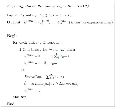
Capacity Based Rounding Method (CBR)
Decision Variables
ztl : Binary variable, 1 if thelth capacity expansion option in Lt is installed on linket∈E ; 0 otherwise , for all t= 1 to m and for alll= 1 to |Lt|
xrijf : Flow passing through path pijf under failure scenario sr , for all i, j∈V :dij0 >0 and forf = 1 to |Pij|and for all sr ∈S
If we relax the binary constraints of the ztl variables and replace them with 0≤ztl≤1 for t= 1 to m and for l= 1 to |Lt|, the resulting problem will be a linear programming problem called the LP-relaxation of our original SNCE. Solving the LP relaxation of any feasible integer programming problem with a minimization objective function provides a lower bound on the optimal objective value.
Here, we like to find a feasible expansion plan for the SNCE problem, by using the optimal solution of the LP-relaxation problem. Let us denote the LP-relaxation problem by LP1. This problem is formulated as follows:
LP Relaxation of Model IP-1 (Model LP1)
M inX et∈E
|Lt|
X
l=1
ctl ztl (6.-1)
subject to.
|Lt|
X
l=1
ztl ≤1 t= 1 to m (6.0)
X
∀i,j∈V:dij>0
|Pij|
X
f=1
ktijfxrijf ≤λtr
ut0+
|Lt|
X
l=1 utlztl
t= 1 to m r = 0 to q (6.1)
|Pij|
X
f=1
xrijf ≥dijr ∀{i, j∈V :dij0>0} r = 0 to q (6.2)