4
REAL-TIME TERRAIN RENDERING
AND VISUALIZATION BASED ON
HIERARCHICAL METHOD
Muhamad Najib Zamri
INTRODUCTION
istory of Geographic Information System (GIS) began since early 20th century saw the development of geographical data information visualization. GIS has changed the people workflow from manual system into an automation system that provides more effective and systematic way. GIS is one of the important developments in the field of information technology where it is a set of computer tools for collecting, storing, retrieving at will, transforming and displaying spatial data from the real world for a particular set of purposes or application domains. Until recently, GIS contributed for many sector and field, including agriculture, archaeology, environmental monitoring, health, forestry, emergency services, marketing, regional planning, site evaluation, tourism and infrastructure.
A complex nature of massive database caused the functionality of traditional GIS (two-dimensional GIS) at its boundary. This conventional system was unable to manage entire information successfully. User interaction with the system only restricted to the operation such as zooming, zoom to extent, panning and picking for viewing and manipulating topographic map. As an alternative, higher dimensional GISs have been proposed to overcome the problem. Three-dimensional Virtual GIS provides a new environment where it attempts to display virtual
scenarios in an appearance identical to the real world. Third dimension facilitates in displaying complex spatial information for visual analysis tasks.
Terrain management and visualization is subfield in 3D Virtual GIS that has attracted a number of researchers to involve in tackling the challenging issues in this research area. In order to display terrain model, computer graphics elements are necessary. Visualization of this 3D model involves large amount of spatial data and imagery data. Thus, it is essential to employ an appropriate optimization algorithm or method to reduce the complexity of problem and at the same time to improve system performance.
Spatial data retrieval technique is one of the solutions for the above-mentioned problem. The objective of this technique is to fetch data rapidly when dealing with real-time massive data. We have designed and developed a terrain management scheme that is based on this technique in order to test the performance of the real-time terrain system.
RELATED WORKS Tile Approach
Pajarola (1998) divided the terrain data into several tiles for an efficient scene management and integrated with the restricted quadtree algorithm. Ulrich (2002) implemented the tile approach for both textures and terrain elevation data in his Chunk LOD.
View Frustum Culling
In view frustum culling, there are two different approaches have been applied: plane intersection test and projection intersection test. First approach needs to compare between six planes of view volume and surfaces of object’s bounding volume. Hoff (1997) has produced rapid axis aligned bounding box (AABB)-view frustum overlapping test in his system. Assarsson and Möller (1999,2000) have presented basic intersection test with four optimization techniques (plane-coherency test, octant test, masking and TR coherency test) for culling AABB and oriented bounding box (OBB).
For the second approach, the comparison merely being made between the projection of view volume and projection of bounding box in screen-space coordinate. Rabinovich and Gotsman (1997) have introduced the concept of union set of projection for bounding box. While Youbing et al. (2001) did not take into account the near, top and bottom planes of view volume in their terrain rendering system for fast determination of terrain patches in each frame.
View-Dependent LOD
TIN-based terrain rendering system has been developed by Hoppe (1998) using his principle of progressive meshes. Unfortunately, this method consumes lot of memory for storing the terrain data.
and Lindstrom and Pascucci (2001) (out-of-core terrain visualization system). Hierarchical quadtree data structure was applied in Röttger et al. (1998) (continuous LOD for height fields) and Ulrich (2002) (ChunkLOD). Hierarchical R-tree also can be used to manage multiresolution terrain data. LOD R-tree has been implemented by Kofler (1998) in his Vienna Walkthrough and Styria Flyover system.
METHODOLOGY Pre-Processing
Pre-processing step is crucial for storing and loading terrain data efficiently as well as obtaining fast data retrieval in real-time environment. In general, the purpose of this phase is to extract the related information and split the terrain data into several patches. Two steps are required: data extraction and data tiling.
Data extraction involves two sequential steps. The first one is the extraction of general information, while the second step is the extraction of elevation profiles. General information is obtained by reading Record A in DEM data format which contains header information about the related USGS DEM data (1992). Certain information will be extracted for facilitating the next process. These include ground coordinates for the corners, minimum and maximum elevation values and column and row data.
Then, according to Record A, the elevation profiles will be read column by column from left to right. The profiles and its related index will be stored in another output file (*.txt file).
Data tiling is the core component of the pre-processing phase. The overlapping tile approach will be used due to its simplicity and seam elimination capability. Therefore, the terrain data must be (2n+1) x (2n+1) in vertical and horizontal directions (Pajarola 1998, Duchaineau et al. 1997, Lindstrom and Pascucci 2001, Röttger 1998, Kim and Wohn 2003).
Firstly, the terrain size needs to be determined in order to ensure the size conform the above rule. There are two suggested steps:
• Find the maximum number of terrain data for one side.
• Assign an appropriate power-of-two plus one (2n+1) value to the maximum number of terrain data for one side.
The terrain data is stored in one-dimensional array which means the index is in the range from 0 to [(2n+1) x (2n+1) - 1]. This approach is applied in order to reduce the memory usage. After calculating and obtaining the terrain size, it is necessary to specify manually the number of vertices per side for each patch. Choosing a proper patch size is depends on data density, CPU speed, available memory and other considerations. Hence, the size must not too small or big for the efficiency purpose. The number of vertices per side must also be in (2n+1) size. The terrain size and number of vertices per side will be used to calculate the number of generated patches for one side as illustrated below:
Then, the starting point for each patch will be determined by computing the index of terrain data. At the same time, a test is made to check the existing status for each patch. It is because when the terrain size is expanded to the (2n+1) x (2n+1), the possibility to generate non-existing patches is high. The purpose of this step is to
reduce the hard disk storage and memory utilization. The existing patches will be assigned with flag 1 and non-existing patches will be assigned with flag 0. Before that, the maximum sizes for vertical (column) and horizontal (row) directions which following the number of vertices per side are needed.
After gaining all basic requirements, the elevation values will be read from the output file that has been created before by searching and comparing the starting point for each existing patches with the index from the output file. Subsequently, normalization of elevation data will be made for each existing patches. Thus, the elevation values will be in range 0 to 255 for facilitating the computation for the run-time process. Minimum and maximum elevation values are required for this computation.
Each patch’s elevation values will be stored in separated output file (*.tile file). This approach is used in order to achieve fast searching and retrieving of terrain patches rather than using single output file with complicated searching process that will slow down the system performance.
Run-Time Processing
Firstly, the view position is needed in order to determine the patches to be processed. The current patch and eight adjacent patches will be selected rather than process the whole terrain patches.
Then, view frustum culling technique is inserted to remove the unseen patches among the nine patches to be processed. Two steps should be followed: plane extraction and intersection test. View frustum comprises of six planes. These planes are left, right, top, bottom, near and far. Each plane has its own plane equation. General plane equation is:
0
The coefficient A, B, C, and D need to be defined in order to complete frustum plane equation. This involves three major steps:
i. Combine the projection and model view matrices. ii. Extract the plane.
iii. Normalize the plane.
Next, the plane-sphere intersection test is made between each view frustum’s planes and terrain patches (bounding sphere representation). Only the terrain patch that has ALL-INSIDE or INTERSECT flag will be taken for the next process. The algorithm is listed below:
Figure 4.1 Pseudo code for plane-sphere intersection test
After that, the tessellations for visible terrain patches are made by using view-dependent LOD algorithm. Röttger’s algorithm (Röttger et al. 1998) has been chosen due to its memory-efficient characterization. It is based hierarchical quadtree structure and managed in top-down manner. In general, the flat and distant objects are given fewer polygons than the close one. The important operations in Röttger’s algorithm involve the distance calculation, subdivision test and generation of triangle fans. All the process in run-time phase are repeated, updated and rendered for each frame.
For i in [all view frustum planes] do Distance = (Center of the sphere X Unit vector) + Coefficient(D) If (Distance > Radius of the sphere) then Return ALL-OUTSIDE
If (Distance > -Radius of the sphere) then Return INTERSECT
End loop
RESULTS
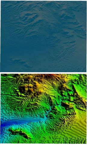
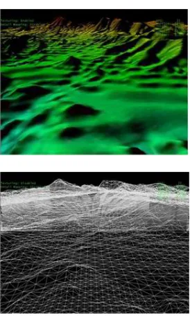
The prototype has been implemented and run on high-end PC in Windows XP operating system. The main specifications are AMD AthlonXP 1800+ (1.53 GHz), 1 GB DDR-RAM and Gigabyte 128 MB ATI Radeon 9700. We have used Arizona data specifically adams mesa area as shown in Figure 4.2 and the results can be seen in Figure 4.3. After running this prototype, average frame rate obtained is 80.53 frames per second (fps), average polygon count is 22370 triangles for each frame and geometric throughput is 15614 triangles per second. For the data accuracy, this system can preserve only 95.34 percent compared to the original full resolution data.
Figure 4.3 Textured and wireframe terrain model
CONCLUSION
REFERENCES
Assarson U. and Möller T., 1999, “Optimized View Frustum Culling Algorithms”, Technical Report:99-3, Chalmers University of Technology, Sweden.
Assarson U., and Möller T., 2000, “Optimized View Frustum Culling Algorithms for Bounding Boxes”, Journal of Graphics Tools, vol. 5, no. 1, pp. 9-22.
Duchaineau M., Wolinsky M., Sigeti D.E., Miller M.C., Aldrich C. and Mineev-Weinstein M.B., 1997, “ROAMing Terrain: Real-time Optimally Adapting Meshes”, Proceedings of IEEE Visualization, pp. 81 – 88.
Hoff K., 1997, Fast AABB/View-Frustum Overlap Test, <http://www.cs.unc.edu/hoff/ research/index.html>.
Hoppe H., 1998, “Smooth View Dependant Level-of-Detail Control and its Application to Terrain Rendering”, Proceedings of IEEE Visualization, pp. 35-42.
Kim S.H. and Wohn K.Y., 2003, “TERRAN: out-of-core TErrain Rendering for ReAl-time Navigation”, EUROGRAPHICS. Kofler M., 1998, “R-trees for Visualizing and Organizing Large
3D GIS Databases”, Technischen Universität Graz, Ph.D. Lindstrom P. and Pascucci V., 2001, “Visua-lization of large
terrains made easy”, Proceedings of IEEE Visualization, pp. 363–370.
Pajarola R., 1998, “Access to Large Scale Terrain and Image Databases in Geoinformation Systems.” Swiss Federal Institute of Technology (ETH) Zürich, Ph.D. Thesis.
Röttger S., Heidrich W., Slusallek P. and Seidel H.P., 1998, “Real-Time Generation of Continuous Levels of Detail for Height Fields”, Technical Report. University¨ Erlangen-N urnberg. Thorsten S. and Anselmo L., 2003, “Simulation of Cloud
Dynamics on Graphics Hardware.” SIGGRAPH/Eurographics Workshop on Graphics Hardware.
Ulrich T., 2002, “Rendering Massive Terrains using Chunked Level of Detail Control”, DRAFT, Oddworld Inhabitants. USGS 1992, “Standards for Digital Elevation Models”. National
Mapping Program Technical Instructions, U.S. Department of the Interior, U.S. Geological Survey, National Mapping Division.