A Study of Numerical Methods for the Level Set Approach
Pierre A. Gremaud∗, Christopher M. Kuster†, and Zhilin Li‡
October 18, 2005
Abstract
The computation of moving curves by the level set method typically requires reini-tializations of the underlying level set function. Two types of reinitialization methods are studied: a high order “PDE” approach and a second order Fast Marching method. Issues related to the efficiency and implementation of both types of methods are dis-cussed, with emphasis on the tube/narrow band implementation and accuracy consid-erations. The methods are also tested and compared. Fast Marching reinitialization schemes are faster but limited to second order, PDE based reinitialization schemes can easily be made more accurate but are slower, even with a tube/narrow band imple-mentation.
1
Introduction
This paper analyzes numerical issues related to the implementation of the level set method for moving interface problems. Let Γ(t),t >0 be a one-parameter family of curves in R2
resulting from the motion of an initial curve Γ(0) under a velocity fieldv. The idea of the level set method, as devised by Osher and Sethian in 1987 [OS88], see also [OF02, Set99b] for more recent reviews, consists in introducing a functionϕ(x, t) that represents the curve Γ(t) as the zero level set of ϕ, i.e., Γ(t) ={x; ϕ(x, t) = 0}. If {x(t), t ≥0} denotes the path of a point on the moving curve, then clearly ϕ(x(t), t) = 0 for t≥0. By taking the time derivative of that last relation, one observes that the function ϕis convected by the velocity fieldv, i.e.
∂tϕ+v· ∇ϕ= 0. (1)
∗Department of Mathematics and Center for Research in Scientific Computation, North Carolina State
University, Raleigh, NC 27695-8205, USA([email protected]). Partially supported by the National Science Foundation (NSF) through grants DMS-0244488 and DMS-0410561.
†Department of Mathematics and Center for Research in Scientific Computation, North Carolina State
University, Raleigh, NC 27695-8205, USA([email protected]). Partially supported by the National Sci-ence Foundation (NSF) through grant DMS-0244488.
‡Department of Mathematics and Center for Research in Scientific Computation, North Carolina State
The vector field v is prescribed on the curve but is arbitrary elsewhere. By decomposing
v into its normal and tangential velocity vn and vτ, it becomes apparent that only the
normal velocity vn =F|∇∇ϕϕ| matters, whereF stands for the normal speed. The level set
equation (1) becomes
∂tϕ+F|∇ϕ|= 0. (2)
Equation (2) is often solved locally near the interface instead of everywhere in space. The advantages of such an approach are obvious in terms of costs and have been discussed at length in the literature, see for instance [AS95, PMO+99]. At each time step, (2) is solved in a tube/narrow band around the current curve. Once the curve, or more precisely the function ϕ, has been updated, the corresponding tube/narrow band is rebuilt. The process then is repeated. It is convenient to initializeϕ(·,0) as the signed distance function to Γ(0). One way to extendF away from Γ(t) is to solve
∇Fext· ∇ϕ = 0, (3)
Fext = F on Γ(t). (4)
Ifφis then evolved according to the extended normal speedFext, i.e.
∂tϕ+Fext|∇ϕ|= 0,
then it is easy to check that ϕ remains a distance function [AS99]. After discretization and/or use of a tube/narrow band implementation, this property may be lost. In many cases, this eventually leads to numerical difficulties, see e.g. [SSO94]. A reinitialization of ϕhas to be applied.
To the authors’ knowledge, accuracy issues related to the use of such tube/narrow band techniques have received far less attention than pure efficiency consideration (through complexity analysis for instance). The accuracy in evolving a moving interface is crucial to many applications. For the level set method, the accuracy depends on two main factors, one is the reinitialization process so that the level set function is not too steep or flat. The other one is the evolution process whose discretization is well understood. A number of efficient methods can be used as part of the reinitialization process. Two such methods are Fast Marching [Set99a] and Fast Sweeping [TCOZ03]. The Fast Marching method is used here.
algorithm is described fully in Section 2. Reinitialization can also be achieved efficiently by using a “PDE-approach” that does not require projection, see for instance [SSO94] or (5) below. Numerical examples and results comparing the efficiency and accuracy of the methods are discussed in Section 3. Conclusions are offered in Section 4.
2
Description of the algorithm
For the sake of simplicity, we consider the initial curve Γ(0) to be a simple, smooth, closed curve inR2. An underlying uniform Cartesian gridThof sizeh is then considered. Assume
we want to follow the evolution of Γ(0) through (2) fromt= 0 to t=T. Approximations Φntoϕat timetn=n∆t,n= 1, . . . , N, ∆t=T /Nand at (some of) the nodes of the mesh
will be successively computed. For stability purposes, the condition ∆t=O(h) is enforced throughout. We denote by Γn(k), the set of the nodes of the mesh within a distance khof
the zero level set of Φn, i.e.
Γn(k) ={P ∈nodes ofTh; dist(P,{Φn= 0})≤ k h}.
The main step of the algorithm consists in going from Φn to Φn+1
n=0 Φ0
= nodal values of ϕ(·,0) while n<N
% PROJECTION
∀P∈Γn
(1) compute dist(P,Γn ) =~Φn
and normal speed ~F % REINITIALIZATION
extend ~Φn
and ~F to Γn (k2) % EVOLUTION
solve (2) from tn
to tn+1 in Γn
(k1) to yield Φn+1 n=n+1
end
In our implementation, we take k1= 5 and k2= 10.
Given a current level set function Φn (which is in general not a distance function),
the PROJECTION step computes the values of the corresponding corrected reinitialized distance function ˜Φn in a domain that is one-layer thick on each side of the interface.
Application dependent techniques have to be used to extend F in that domain. In the present implementation, the REINITIALIZATION step is done through a second order Fast Marching method (see subsection 2.2), or the PDE approach. Finally, the EVOLUTION is done by a classical WENO scheme (see subsection 2.3).
Φnis considered as an initial value for the problem
∂¯tϕ+ sign(Φn)(|∇ϕ| −1) = 0, (5)
which is to be solved to steady state as the fictitious time ¯t→ ∞, where sign is a smoothed sign function, see [SSO94] for example. Often, a good approximation of the distance function is good enough and only a few iterations are needed if the computational domain is large enough. This approach has the merit of being simple however, it may not be very efficient (for instance, not taking enough time steps may result in severe losses in accuracy if the computational tube is thin).
2.1 Computing the orthogonal projections
Before we apply the fast marching method for reinitialization process, we need to know a good approximation of the distance function within one grid size of the interface, that is, within Γn(1). This can be done in various ways.
2.1.1 A direct approach from a quadratic equation.
A simple third order method has been proposed in [HLOZ97, LZG99]. This method is third order accurate and “direct”, i.e., no iterations are needed.
Assume that x is a grid point near the interface. LetX∗ be the orthogonal projection ofx on the interface. Considering the Taylor expansion ofϕat x, we have
0 = ϕ(X∗)
= ϕ(x) +∇ϕ(x)·(X∗−x) +1 2(X
∗−x)THe(ϕ(x))(X∗ −x) +O(|X∗−x|3),
where He is the Hessian matrix ofϕ. For xclose to the interface,
X∗−x≈α∇ϕ(x), for someα∈R.
This leads to the following quadratic equation forα
0 = ϕ+α|∇ϕ|2+α
2
2 ∇ϕ
THe(ϕ)∇ϕ,
= ϕ+α(ϕ2x+ϕ2y) +
α2 2 (ϕxxϕ
2
x+ 2ϕxyϕxϕy +ϕyyϕ2y),
where the above functions are all evaluated at x. If the derivatives are approximated by standard five-point finite difference formulas, then the projection method is third order accurate, i.e.
2.1.2 A constrained minimization method
We also propose a projection method based a constrained minimization problem. This method has the same order of accuracy as the direct method mentioned above, gives slightly better results (that is, with smaller error constant) and has about the same cost. For any nodeP = (x0, y0)∈Γn(1) where the distance function is to be evaluated, we construct the
unique polynomialqP inQ2 = span{1, x, y, xy, x2, y2, x2y, xy2, x2y2} agreeing with Φn at
the 9 point centered at P, see Appendix A for details. For the present purpose, Γn(1) is
taken as to contain nodes admitting neighbors of opposite sign, but also neighboring nodes of values less than h2. The square of the Cartesian distance,kx−x0k2 is then minimized
subject to the constraintqP = 0. The Lagrangian for this problem is
L(x, y, λ) = (x−x0)2+ (y−y0)2+λ qP(x, y). (6)
To find the point (x, y), we solve the system
∇L(x, y, λ) = 0, (7)
i.e.,
2(x−x0) +λ∂qP(x, y)
∂x = 0
2(y−y0) +λ
∂qP(x, y)
∂y = 0
qP(x, y) = 0.
(8)
Newton’s method is used to solve this nonlinear system; then the value of Φ atP is set to be the distance between that point and the solution. The sign of the distance function at each point is taken to be the same as the sign of the current level set. Finally, the gradient at each point near the interface is computed using centered differences on the level set and then normalizing the result so that the gradient has magnitude 1.
2.1.3 Other approaches
A method suggested in [LFO95] involves starting at a mesh pointxij and repeatedly taking
a step, in the direction of the (negative) gradient, of length given byϕat the current point. The loop is terminated when |ϕ| is small enough. It is noted [LFO95] that this process does not always converge: if the onset of divergence is detected (|ϕ| larger than some predetermined magnitude) or if too many iterations are taken, a different method is used (see [LFO95] for details). Another method, used by Chopp [Cho01], constructs local bi-cubic approximations. Newton’s method is then used to find points on the zero level set of those functions. Note that for both of those methods, what is minimized is an approximate functionϕrather than a genuine distance.
simpler than the one discussed in [ELF05], has a higher asymptotic rate of convergence and has comparable conservation properties, see Section 3.
2.2 Reinitialization and Fast Marching
The Fast Marching algorithm, first introduced by Tsitsiklis [Tsi95] and then popularized by Sethian and his coworkers, see e.g. [Set99a], is a single-pass Dijkstra-like algorithm de-signed to solve graph traversal problems. This algorithm calculates the nodes in a smallest first ordering by using a Heap Sort to keep track of the current smallest valued node. The Heap Sort data structure is order log(M) for insertions, deletions, and updates whereM is the total number of nodes in the domain. The use of this data structure, along with the single-pass nature of the algorithm, means that the algorithm as a whole is orderMlog(M) .
Here, the Fast Marching method is used to compute the distance function and the extension of the normal speedFext, see (3), in a tube/narrow band around the interface
by solving the Eikonal equation
|∇ϕ| = 1, (9)
ϕ = 0 on Γ(t), (10)
for ϕ and solving (3,4) for Fext. A second order discretization is used for solving (9,10)
as described below. The system (3,4) is discretized at first order. Following the method described in [SV00, SV03] on a Cartesian grid, consider a node X0 at which the solution
ϕ is to be computed and two neighboring nodes X1 and X2 at which the values of ϕ
(ϕ`, ` = 1,2) and its derivatives (∂xϕ`, ∂yϕ`, ` = 1,2) are known or have already been
computed. We define
N`=
X0−X`
|X0−X`|
, `= 1,2 and N =
N1
N2
,
The directional derivatives in the directionsN1 andN2 are approximated to second order
by
D`ϕ= 2
ϕ0−ϕ`
|X0−X`|
−N`·[∂xϕ`, ∂yϕ`] `= 1,2.
Those approximate directional derivatives are linked to the gradient by
D`ϕ=N`· ∇ϕ+O(|X0−Xi|2) or Dϕ=N ∇ϕ+O(h2), (11)
whereDϕ= [D1ϕ, D2ϕ]. Using the fact that NtN =I on the present Cartesian grid and
plugging into (9), the following quadratic equation forϕ0 is obtained
If the value of ϕ is only known at a single neighboring node,X1, then the gradient is
assumed to lie entirely along the line connecting X1 and X0. If this is the case, then the
following relation is used
ϕ0 =ϕ1+h (13)
2.3 Evolution
A third order total variation decreasing (TVD) Runge-Kutta scheme [GS98] coupled with a third order WENO scheme for the spatial derivative [JP00]. The method solves numerically the differential equation
∂tϕ=L(ϕ). (14)
by
ϕ(1) =ϕn+ ∆tL(ϕn),
ϕ(2) = 3 4ϕ
n+1
4ϕ
(1)+1
4∆tL(ϕ
(1)),
ϕn+1 = 1 3ϕ
n+2
3ϕ
(2)+2
3∆tL(ϕ
(2)).
(15)
whereL(ϕ) is the WENO approximation ofv· ∇ϕ. A time step of ∆t= ∆/(2smax) where
smax is the absolute maximum normal speed in the tube/narrow band was used.
10−4 10−3 10−2 10−1
10−8 10−7 10−6 10−5 10−4
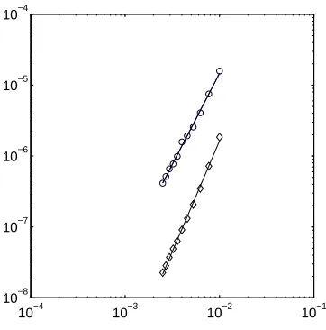
Figure 1: Constant expansion using Fast Marching with projection from 2.1.2: L1 (dia-mond) and L∞ (circles) rates of convergence in the tube/narrow band under grid
3
Numerical examples
All tests were performed using a 1.2 GHz PowerPC G4 processor with 768 MB of DDR SDRAM. The results given below have been computed using the algorithm described above with various projection methods. TheL1 andL∞errors are computed in the tube/narrow band (a trapezoidal rule is used for the calculation of theL1error). The error is taken here
in terms of level set functions, i.e., it is the difference between the exact distance function to the final curve and its numerical approximation (this requires a “final” reinitialization). By the very nature of the present tube/narrow band method, the computational domain shrinks with h. A third order method with respect to the L1 norm as measured above is in fact second order on a fixed domain.
In the PDE approach, the level set functions are not reinitialized to the signed distance function and the error is measured from the computed orthogonal projections.
3.1 Constant Expansion
The first example is a circle expanding/shrinking along the normal direction, that is
v = F(t)n, where n is the unit normal direction. The results are shown for F(t) = 1. This simple case is in fact representative: results for more general functionsF(t) are com-parable. For the Fast Marching method with projection from 2.1.2, the L1 and L∞ rates of convergence of order are found to be roughly 3 (3.14) and slightly above 2 (2.58), re-spectively, see Figure 1. Again, this corresponds to a second order method inL1 on a fixed spatial domain.
1/h PDE rate Taylor rate Min. rate
100 .738 – .418 – .435 –
160 3.07 3.03 1.08 2.02 1.11 1.99
220 7.78 2.92 2.23 2.28 2.27 2.25
280 16.2 3.04 4.00 2.42 4.16 2.52
340 28.9 2.98 6.46 2.47 6.66 2.42
400 47.1 3.01 10.1 2.75 9.96 2.48
Table 1: CPU time (in seconds) versus size of the mesh. The above rates refer to α, where time=O(h−α)for the PDE approach (5), the Fast Marching method with projections from
2.1.1 (Taylor) and from 2.1.2 (Min.) respectively.
in the band is of order O(1/h). Therefore, at each time step, the PROJECTION and REINITIALIZATION steps cost O(1/hlog 1/h) by the standard complexity analysis of Fast Marching. As there areO(1/h) time steps by stability, the total number of operations for the algorithm is of orderO(1/h2log 1/h). This crude analysis is confirmed by the result of the above Table 1. In the PDE approach, we do the reinitialization and solve the level set equation (5) in the entire domain (O(1/h2) operations), however, only one reinitialization
step is carried out (in ¯t, see (5)) for each time step in (2). The total number of operations for the PDE approach on the entire domain is thus of order O(1/h3), an observation that also confirmed in Table 1.
In Table 2, we show a grid refinement analysis of different methods for the expanding circle. To compute the error, each node in ΓN(1) is numerically projected onto the current
curve; the error reported in Table 2 corresponds to the maximum distance between those projected points and the exact curve.
1/h PDE rate Taylor rate Min. rate
100 4.09(-6) – 1.01(-5) – 7.53(-6) –
160 1.26(-6) 2.51 2.60(-6) 2.89 2.06(-6) 2.76 220 4.75(-7) 3.06 1.35(-6) 2.06 1.11(-6) 1.94 280 2.40(-7) 2.83 7.10(-7) 2.66 6.06(-7) 2.51 340 1.36(-7) 2.93 4.92(-7) 1.89 3.99(-7) 2.15 400 7.58(-8) 3.60 3.67(-7) 1.80 2.93(-7) 1.90
Table 2: Constant expansion: L∞-error of the projection for the PDE approach, the “Tay-lor” approach from 2.1.1 and the minimization method of 2.1.2.
In this trivial example, all methods converge with the expected rate, three for the PDE approach (on the full spatial domain) thanks to the use of the third order TVD WENO-RK scheme (15) and two for the Fast Marching based algorithms in spite of the narrow band implementation.
3.2 Rotations
The second example is the rotation of an off center circle. Initially, the circle is (x−0.5)2+ y2 = 0.252. The velocity field is v= (y,−x). The errors are measured after one complete rotation.
1/h PDE rate CPU PDE-tube rate CPU Taylor rate CPU Min. rate CPU 64 4.86(-3) – 26.6 5.26(-3) – 23.8 6.04(-3) – 3.76 5.70(-3) – 3.87 128 1.90(-4) 4.68 220 1.90(-4) 4.79 115 4.90(-4) 3.62 19.2 4.06(-4) 3.81 19.7 256 9.87(-6) 4.27 1808 1.07(-5) 4.15 675 1.20(-4) 2.03 118 9.07(-5) 2.08 119 512 1.33(-6) 2.89 14555 1.51(-6) 2.82 4167 2.63(-5) 2.19 900 2.16(-5) 2.07 900
Table 3: Rotation of an off center circle: L∞-errors, convergence rates and CPU times (in
seconds) after one complete rotation.
many reinitialization steps are needed, usually int(δ/h) steps so that the reinitialization process reaches the tube boundary. The error is measured from all the orthogonal pro-jections of Γn(1), i.e., of the first layer of nodes. Note that for the PDE approach, the
level set function may not be a good approximation of the signed distance function. But this does not bring inaccuracy to the level set method as long as the level set function remains smooth and well-behaved (not too steep or flat) near the front. The computed orthogonal projections within one grid size of the interface is third order accurate. In Ta-ble 3, PDE refers to the PDE approach in the entire domain while PDE-tube corresponds to that approach in a narrow band of width 10h. For both versions, the PDE approach is again observed to be third order accurate but is significantly slower than the Fast Marching method with either projection.
−1 0 1
−1 1
0
−1 0 1
−1 0 1
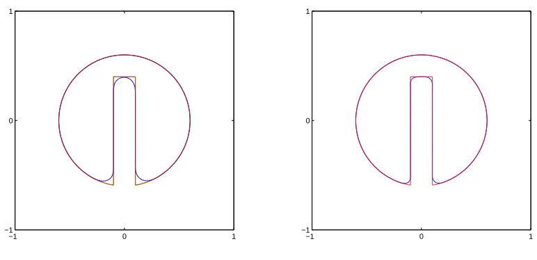
The third example is a single rotation of the shape (called Zalesak’s disk) shown in Figure 2. In this example, the velocity field is taken as fixed,v= (y,−x). No extension of F was taken. This example is similar to the one used in [ELF05] and other publications.
10−4 10−3 10−2 10−1 100 10−5
10−4 10−3 10−2 10−1
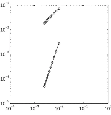
Figure 3: Rotation of Zalesak’s disk with Fast Marching with projection from 2.1.2: L1
(diamond) and L∞ (circles) rates of convergence in the tube/narrow band under grid re-finement: L1-rate ≈2.93, L∞-rate ≈1.01.
For Fast Marching with projection from 2.1.2, the L1 and L∞ rates of convergence of order in the tube/narrow band are found to be roughly 3 (2.93) and 1 (1.01), respectively, see Figure 3. The order 1 convergence in the maximum norm is consistent with the presence of “shocks” (discontinuities in the first derivatives) for the present example.
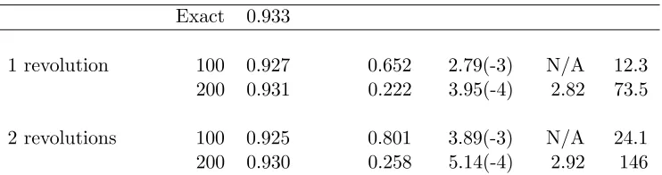
Grid Cells Area % Area loss L-1 Error Order CPU Exact 0.933
1 revolution 100 0.927 0.652 2.79(-3) N/A 12.3
200 0.931 0.222 3.95(-4) 2.82 73.5
2 revolutions 100 0.925 0.801 3.89(-3) N/A 24.1
200 0.930 0.258 5.14(-4) 2.92 146
Table 4: Area loss, L1 errors and rates and CPU time (in seconds) for the Zalesak’s disk rotation problem for Fast Marching with projection from 2.1.2.
4
Conclusions
Fully second order numerical methods for the reinitialization and evolution processes of a level set function are investigated. The methods result from the combination of (i) an accurate process to find the orthogonal projections at grid points directly next to the interface, (ii) a second order Fast Marching method and (iii) a third order TVD WENO-RK scheme. For computational efficiency, all calculations are made only in the neighborhood of the current curve (tube/narrow band) for this approach.
A qualitative analysis and comparison between a high order PDE approach and the above Fast Marching based methods are given. Both types of methods are found to work well, the latter ones being faster, better suited to tube/narrow band implementation but limited to second order.
References
[AS95] David Adalsteinsson and James A. Sethian,A fast level set method for propagat-ing interfaces, J. Comput. Phys.118 (1995), no. 2, 269–277. MR MR1329634 (96a:65154)
[AS99] D. Adalsteinsson and J. A. Sethian,The fast construction of extension velocities in level set methods, J. Comput. Phys.148(1999), no. 1, 2–22. MR MR1665209 (99j:65189)
[Cho01] David L. Chopp, Some improvements of the fast marching method, SIAM J. Sci. Comput.23(2001), no. 1, 230–244.
[GS98] Sigal Gottlieb and Chi-Wang Shu, Total variation diminishing Runge-Kutta schemes, Math. Comp.67(1998), no. 221, 73–85. MR MR1443118 (98c:65122)
[HLOZ97] T. Hou, Z. Li, S. Osher, and H. Zhao, A hybrid method for moving interface problems with application to the Hele-Shaw flow, Journal of Computational Physics134 (1997), 236–252.
[JP00] Guang-Shan Jiang and Danping Peng, Weighted ENO schemes for Hamilton-Jacobi equations, SIAM J. Sci. Comput. 21 (2000), no. 6, 2126–2143 (elec-tronic). MR MR1762034 (2001e:65124)
[LFO95] Frank Losasso, Ronald Fedkiw, and Stanley Osher, Spatially adaptive tech-niques for level set methods and incompressible flow, Computers and Fluids (1995), In Press.
[LZG99] Z. Li, H. Zhao, and H. Gao, A numerical study of electro-migration voiding by evolving level set functions on a fixed cartesian grid, Journal of Computational Physics152 (1999), 281–304.
[OF02] S. Osher and R. Fedkiw, Level set methods and dynamic implicit surfaces, Springer, 2002.
[OS88] Stanley Osher and James A. Sethian, Fronts propagating with curvature-dependent speed: algorithms based on Hamilton-Jacobi formulations, J. Com-put. Phys.79(1988), no. 1, 12–49. MR MR965860 (89h:80012)
[PMO+99] Danping Peng, Barry Merriman, Stanley Osher, Hongkai Zhao, and Myungjoo Kang,A PDE-based fast local level set method, J. Comput. Phys. 155 (1999), no. 2, 410–438. MR MR1723321 (2000j:65104)
[Set99a] J. A. Sethian,Fast marching methods, SIAM Review 41(1999), 199–235.
[Set99b] , Level set methods and fast marching methods, second ed., Cambridge Monographs on Applied and Computational Mathematics, vol. 3, Cambridge University Press, Cambridge, 1999, Evolving interfaces in computational geom-etry, fluid mechanics, computer vision, and materials science. MR MR1700751 (2000c:65015)
[SSO94] Mark Sussman, Peter Smereka, and Stanley Osher, A level set approach for computing solutions to incompressible two-phase flow, J. Comput. Phys. 114
(1994), 146–159.
[SV00] J. A. Sethian and A. Vladimirsky, Fast methods for the eikonal and related Hamilton-Jacobi equations on unstructured meshes, Proc. Natl. Acad. Sci. USA
[SV03] James A. Sethian and Alexander Vladimirsky, Ordered upwind methods for static Hamilton-Jacobi equations: theory and algorithms, SIAM J. Numer. Anal. 41(2003), no. 1, 325–363 (electronic). MR MR1974505 (2004f:65161)
[TCOZ03] Y. R. Tsai, L-T. Cheng, S. Osher, and H. Zhao,Fast sweeping algorithms for a class of Hamilton-Jacobi equations, SIAM Journal of Numerical Analysis41
(2003), 673–694.
[Tsi95] John N. Tsitsiklis, Efficient algorithms for globally optimal trajectories, IEEE Trans. Automat. Control 40 (1995), no. 9, 1528–1538. MR MR1347833 (96d:49039)
A
Q
2Coefficients
Given a Cartesian grid discretization, a 9 point stencil around the point xij can be used
to approximateϕ(x) as a uniqueQ2 function in the vicinity ofxij. This is done by solving
the linear system
a0+a1xk+a2yl+a3xkyl+a4x2k+a5y2l +a6x2kyl+a7xky2l +a8x2kyl2 =ϕ(xk, yl) (16)
wherek =i−1. . . i+ 1 and j=j−1. . . j+ 1. This is a set of 9 linear equations with 9 unknowns. If the local discretization is translated and scaled such that xij = (0,0), and
the grid size is,h= 1, then one finds
a0 =ϕij
a1 = (ϕ(i+1)j−ϕ(i−1)j)/2
a2 = (ϕi(j+1)−ϕi(j−1))/2
a3 = ((ϕ(i+1)(j+1)−ϕ(i−1)(j+1))−(ϕ(i+1)(j−1)−ϕ(i−1)(j−1)))/4
a4 = (ϕ(i+1)j−2ϕij+ϕ(i−1)j)/2
a5 = (ϕi(j+1)−2ϕij+ϕi(j−1))/2
a6 = ((ϕ(i+1)(j+1)−ϕ(i+1)(j−1))−2(ϕi(j+1)−ϕi(j−1))
+ (ϕ(i−1)(j+1)−ϕ(i−1)(j−1)))/4
a7 = ((ϕ(i+1)(j+1)−ϕ(i−1)(j+1))−2(ϕ(i+1)j−ϕ(i−1)j)
+ (ϕ(i+1)(j−1)−ϕ(i−1)(j−1)))/4
a8 = ((ϕ(i+1)(j+1)−2ϕ(i+1)j +ϕ(i+1)(j−1))−2(ϕi(j+1)−2ϕij+ϕi(j−1))
+ (ϕ(i−1)(j+1)−2ϕ(i−1)j+ϕ(i−1)(j−1)))/4.