A time-saving method to compute multi-pass weld residual stresses

A

Dr-Eng

Dr-Eng

it remain compone This is du full 3D co D simplified the “macr instead o only for a Rossillon particular procedure experime R (Rossillon computat simulatio During ou only the reproduct welded ar I numerica

A TIME S

g, EDF SEPT

g, EC2-Modé

ACT In order to ob ding has prov xt of engineer ith reasonable ensuring an ac The method c ately selected metrical param ely studied in nd to literature mputation time

nfigurations th

DUCTION To have a bet operation are on of welding

d during weldi ng experimen

al. (2009), Mu ns a difficult t

nts such as p ue to the high omputations a Despite recen d methods to ro-bead” tech f analyzing th a few “macro-n a“macro-nd Deprade rly concerning e usually requ ental measurem Recent invest n and Deprad tion. Among t ons (Brickstad ur investigatio last deposited tion of the str rea, even in ca In this paper, al or experim

SAVING M

Fré

TEN,Villeur

élisation, Vil

btain the residu ved efficient a

ring studies, i e computation ccurate reprod consists in inc

passes. For a eters. The me n the literature e results, are v es divided by han girth-weld

tter assessmen e investigated has become ing, and a goo ntal versus nu

uranski et al.

task to compu pressure vesse

number of pa are required. nt progresses compute wel hnique, which he thermo-me -beads”. This eux (2011)). H

g the determi uires some fi ments. Moreov tigations on m deux (2011)) s these, the idea and Josefson ons on welded d bead, or of ress field. Thi ases for which we focus only mental solution

METHOD

RESID

édérique Ros

rbanne, Franc

lleurbanne, F

ual stress field and has becom it remains a d n times. In thi duction of the cluding in the

given materia ethod is applie and standard very satisfacto

a factor comp d pipes, and m

nt of the in ser d. Since majo a very intere od alternative merical result (2011), and O ute residual s els of PWR’s, asses involved

in the field ld residual str

consists in m chanical resp enables to red However, this ination of the itting of the m ver, the choic multi-pass weld

showed some a of simulating n (1998)), seem d divider plate

a few approp is was observ h a large numb y on weld resi ns exist in th

D TO CO

DUAL ST

ssillon

and

ce (frederiqu

France

d resulting fro me an interesti difficult task to

is paper, a tim residual stres e simulation o al and a given ed to various g s. The results, ory. Quasi-ide prised betwee more complex 3

rvice loading o or developmen esting and stra to measurem ts have demon Ogawa et al..(

tresses with r , weld residua d, and also to

of parallel c resses by FE s merging togeth

onse for every duce computat

technique, th e heat inputs t

model data in e of the macro ding computa

promising tra g only the las ms very intere es, it was how priately select ved not only i ber of passes w

idual stresses he open litera

OMPUTE

TRESSES

Lionel Dep

ue.rossillon@

om the welding ing alternative o compute res me-saving met

s field with dr only the last heat input, th geometries of , confronted to entical residua

n 7 up to 12. 3D geometry

of PWR comp nts have been aightforward ments. A large nstrated the re (2009). Howev reasonable co al stresses are the complex g

computation, simulations. A

er two or mor y weld pass, t tion times on hough adequat that have to b n order to rep o-bead is often ations on the w ails concerning st bead, somet

sting, but is n wever observed

ted passes, co in the vicinity was involved.

in pipe girth ature. Moreov

MULTI-S

radeux

@edf.fr)

g process, num e to practical sidual stresses thod is propos rastically redu deposited pas he choice of re f austenitic pip o multi-pass s al stress fields Further comp like J welds.

ponent, residu n achieved in means of pre amount of ac elevancy of w ver, in the con omputation tim e difficult to c geometry of th

engineering Among these

re passes into the numerical 3D geometrie te in some cas be considered produce accu n arbitrary. welded divider

g simplified m times consider not always suit d that, in man ould be suffic y of the last b .

welds, for wh ver, the weld

-PASS WE

merical simula measurement s for a very hi sed to comput uced computin ss, or a reduc emaining pass pes girth weld simulations in

are computed putations are i

ual stresses ge n this field, ediction of res

ademic or ind weld numerica ntext of engine mes. In partic

compute by F he welded are

departments methods, a co

one weld blo l simulations es (see Watson ses, shows som d in the macr urately numeri

r plates of ste methods of re red in early w table for very ny cases, the c cient to ensure

bead, but also

hich many wel d residual stre

ELD

ation of multi t. However, in igh number o te the welding ng times. ced number o ses depends on ds, which have cluding all the d in both case

in progress on

enerated by the finite elemen sidual stresse dustrial studie al simulations eering studies ular, for thick FE simulation eas. Therefore

still resort to ommon one i ock. Therefore are performed n et al. (2006) me limitations o-beads. Such ical results o

eam generator sidual stresse weld numerica deep grooves computation o e a very good o in the whole

phenomena in such structures are well understood (Bouchard (2007), Legatt (2008), Dong (2007)). In addition, numerical investigations on such configurations can be performed with 2D axisymetrical models, which require low CPU times. Therefore, the method could be evaluated rather quickly on such geometries, before investigating more complex cases with 3D geometries.

Different numerical test cases have been defined, in order to cover a wide range of configurations, with various numbers of passes. Then a complete multi-pass weld simulation is performed for each test, in order to settle a reference residual stress field. This reference solution is then validated by comparison with existing numerical-experimental solutions from the literature on similar configurations. Afterwards, different simplified simulations are detailed and compared to the reference results, including the simulation of only the last bead instead of the totality. The results are then discussed. Finally, a practical selection procedure of the passes that must be taken into account in the analysis is proposed, based on mechanical and geometrical criteria.

TESTS DEFINITION

The test cases are typical of pipe girth welds configurations. The study focuses only on austenitic stainless steel pipes, in order to avoid solid-state phase transformation consideration. , In the past two decades, residual stresses in austenitic pipe girth welds have been widely investigated, using either experimental and-or numerical methods, generally toward a goal of fracture mechanics based defect assessment (Stacey et al.(2000)), or on purpose of corrosion investigation. A great amount of results is currently available in the open literature for different weld pipe configurations and for various materials. These results led to compilations of through-wall residual stress distributions such as those given in assessment code procedures (Lee and Chang (2008)). More recently, the development of weld numerical simulations by FE method led to the generalization of parametric studies allowing a deep comprehension of residual stress formation mechanisms in pipes. As a result, synthetic papers as those of Dong (2007) highlighted the parameters (mainly geometrical) governing the residual stress distribution in pipes and vessels girth welds. In parallel, other works, as those of Bouchard (2007), made critical reviews of existing through-wall residual stress distributions, and proposed accurate residual stress profiles for different configurations. These profiles were corroborated by measurements using various methods. It should be pointed out that, despite the good knowledge of residual stresses in pipes, multi-pass welding simulation in pipes are still relevant in the industry at least for two reasons: firstly, some particular restraint conditions may invalidate the recommended residual stress profiles (Legatt (2008)), and numerical simulation is helpful to take into account special boundary conditions; Secondly, some special welding procedures might require a full 3D analysis to catch the gradient along the circumference of the pipe (Lee and Chan (2008)).

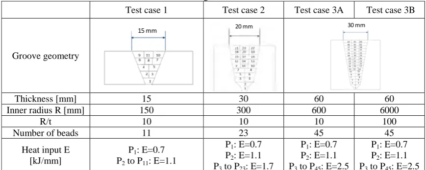
The test cases geometries have been defined so as to cover the entire range of residual stresses distributions in austenitic weld pipes (from “bending type” to “self-equilibrated type” according to Dong (2007), and to remain close enough to well-documented solutions (either experimental, numerical or both) of the open literature. The geometry and heat input parameters are summarized in figure 1 and 3. The heat input parameters are typical for such kind of configurations.

Table 1: Configuration of the tests

Test case 1 Test case 2 Test case 3A Test case 3B

Groove geometry

Thickness [mm] 15 30 60 60

Inner radius R [mm] 150 300 600 6000

R/t 10 10 10 100

Number of beads 11 23 45 45

Heat input E [kJ/mm]

P1: E=0.7

P2 to P11: E=1.1

P1: E=0.7

P2: E=1.1

P3 to P23: E=1.7

P1: E=0.7

P2: E=1.1

P3 to P45: E=2.5

P1: E=0.7

P2: E=1.1

P3 to P45: E=2.5

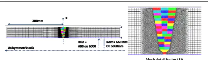
Figure 1: Mesh details for test 3 A and B

REFERENCE MULTI-PASS COMPUTATION

For each test, the reference results are obtained by a multi-pass computation using a classical FE welding simulation. The computation is performed with the FE Code Code_Aster® developed by EDF. The mesh and the weld details are shown in fig. 1. Each pass is computed individually and is included in the model gradually according to the weld sequence (see Table 1). At first, the thermal analysis is performed and the time-dependent temperature field is saved for the subsequent mechanical analysis. The transient temperature history is computed by solving the heat conduction equation, assuming temperature-dependent physical properties. The latent heat of fusion is neglected, as it has proven to have negligible effect on the result. The weld passes are included in the model gradually following their deposition.

The heat input is described as an internal volumetric body heat source, prescribed in each bead individually. This body heat source is constant in space over the bead, but vary linearly with time, in order to reproduce the approaching and moving away of the welding torch. This description of the heat input allows calibrating the parameters tm and max for a given prescribed heat input, as follows:

(1)

In the Eqn. 1, fixed values of tm and of the heat input E give directly the value of max. Then, knowing the

heat input E, there is only one parameter, only tm has to be adjusted. The parameter is then fitted to ensure a

maximal temperature equal or exceeding the fusion temperature in all points of the bead. This method has proven its efficiency on other studies, by comparisons with full 3D simulations including more complex moving heat sources. It is now commonly used in EDF studies (Rossillon and Depradeux (2011)).

Radiative and convective heat exchanges with the environment are also taken into account. However, these parameters have a weak effect on the thermal results, as heat conduction in the pieces is the main heat exchange phenomenon. After the thermal transient computation, the mechanical analysis is performed with the thermal history as an input for the thermal strain computation using temperature-dependent material properties. An elasto-plastic model with linear kinematic hardening, and temperature-dependent material properties, is considered, with classical values for austenitic steel.

For simplification purpose, it is assumed that the weld deposit and the base material have the same mechanical properties as the base metal. Despite the yield stress mismatch between the weld and the parent material could possibly affect the results in some ways, it does not change the overall through-thickness residual stress distribution as demonstrated by Dong (2007), and this can be excluded from the analysis. It is also demonstrated that the t and R/t ratio are the critical parameters for the stress distribution.

The reference solutions for the stress field, calculated for each tests, are given on fig. 2:

a) Test 1 exhibits a typical “bending” stress pattern, with an inversion of the sign of the stress through the thickness at the center of the weld, and a “mirror” pattern of the axial stress profiles along the pipe axis between the outer and the inner surfaces. On the contrary, the hoop stresses are more uniform through the thickness, with tensile stresses near the weld, and compressive stresses surrounding the weld area

b) Test 2 presents a less pronounced bending stress pattern, as the hoop restraint is counterbalanced by the axial one. This is due to the large thickness of the pipe. As a result, less tensile stress are generated at the inner surface

c) Test 3A and B exhibit both typical “self-equilibrated” stress patterns, with compressive axial stresses in the middle of the thickness. However, the radius influence is clearly visible on the inner surface of the pipe, for both hoop and axial stresses.

Figure 2: Reference results obtained with a complete bead by bead analysis for each tests

Figure 3: Comparison of stress profiles calculated with Code_Aster with results of the literature for test case 1, 2 , 3A and 3B.

Simulation, t=15 ; R/t=10 Test –case1

Dong (2007) t=16 ; R/t=25 ; X weld

Simulation

t=60 ; R/t=10  or 100 ; V weld Test –case 3A and 3B

Bouchard (2007) t=62 ; R/t=3 ; MMA weld

Test –case2 – hoop stress

Deng et al.(2008) Simulation ‐t=30; R/t=10; 

Simulation ‐t=30; R/t=10; 

Deng et al.(2008)

The results have been compared with a panel of literature results on similar configurations (Bouchard (2007), Legatt (2008), Dong (2007) and Deng et al. (2008). It showed a very good agreement, accrediting the relevancy of our computation procedure. As an example,the left-upper side of Figure 3 compares the results for test 1 with different profiles taken from Dong (2007). A typical axial stress pattern is observed for that configuration.

The down part of Figure 3 also compares the results from test 2 with the results from Deng et al. (2008) on a similar configuration (austenitic pipe, 14 beads, t=23 mm, R=85 mm, E = 1 to 3 KJ/mm). The computed stress profiles show very good agreement with the experimental and numerical results from Deng et al. (2008), although the material data, heat input and geometry are slightly different.

Results of the through-wall stress evolution along the thickness for test 3A and 3B are also compared with results from Bouchard (2007) on fig. 3 (right-upper side). The overall computed evolutions are similar to literature’s results on such kind of configuration, though the R/t values are larger on test 3A and 3B than in the cases considered in Bouchard (2007). Moreover, higher heat input is responsible for a larger zone of stress decrease at the approach of the outer surface, for both tests 3A and 3B. This tendency is confirmed by the available measurements.

SIMULATIONS WITH SIMPLIFIED METHOD

The principle of the method is to select the last bead, or a small number of appropriately selected beads, and to run the simulation of welding in the same way as for the multi-pass calculation, but only for the retained beads.

For test cases 1 and 2, only the last bead deposit has been considered in the numerical analysis. This means that at the initial state, all the beads except the last one are present in the FE model, but with zero stress or displacement. Only the deposit of the last bead is computed, with exactly the same methodology as for the multi-pass calculation previously presented. In particular, the heat input prescribed in the selected bead is the same as it would have been in the complete multi-pass analysis.

The corresponding results of the simplified analyses for tests 1 and 2 are confronted to the results of the reference multi-pass simulations on figure 4 and 5. The results are quite interesting: the stress states are almost exactly the same for the simplified methods as they would have been for the complete multi-pass ones. In addition, figure 5 shows that the results for tests 1 and 2 are also very close to literature results, strengthening the robustness of the analyses.

For both tests (1 and 2), the simulation of the last bead only is sufficient to reproduce the stress gradients and maximum, not only at the surface of the pipe, but also through the thickness. This is particularly interesting for test 2, as the obtained results with a single bead computation are almost the same as the numerical (and experimental) ones obtained in Deng et al. (2008) with a 14 passes computation.

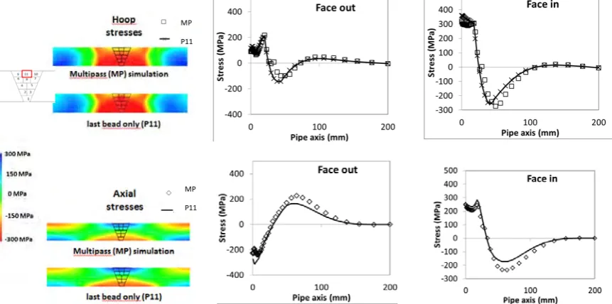
Figure 4: Comparison between the multi-pass simulation (MP) and the simplified method (P11) for test 1

MP

P11

MP

Figure 5: Comparison between the multi-pass simulation (MP) and the simplified method (P23) for test 2

However, as expected, in test cases 3A and 3B for which the thickness is larger, the simulation of the last deposited bead only, fails to reproduce accurately the stress state obtained by the complete multi-pass simulation. A closer look at the plastic zone shows that there is a close relationship between the spatial distribution of the weld residual stresses in the circumferential direction, and the shape of the plastic zone around the bead (figure 6).

Figure 6: Size of the plastic zone and hoop stresses calculated for the last bead only on test 3A

Following this observation, if one consider only a few intermediate passes in the thickness, it seems possible to cover the plastic zone of the entire weld joint. The idea is to cover the same plastic zone as the one that would be generated by the whole bead by bead simulation. In order to determine which bead will be selected in the simulation, one has to consider the size of the plastic area around each bead. Assuming a cylindrical distribution of the plastic zone around the bead, the radius of the zone can be estimated by the following equation (R6 (2004)):

ܼܴܲ ൌ ට

ೊ௘గఘ஼

ொ

௏

(2)

If the value of PZR is larger than the thickness of the wall, the last deposited layer only can be retained, and the deposit of the other ones may be neglected in the analyses. Moreover, if the last layer contains only a small number of beads, and that the last bead is deposited in the center of the layer (as for the present test cases), only the last bead could be considered. On the contrary, if the last layer is composed of a large number of beads, the beads located at both sides of the layer should be taken into account in order to reproduce accurately the axial stress gradients along the outer surface.

For test cases 1 and 2, the radius of the plastic zone is larger than the thickness of the pipe, and therefore, the last bead is sufficient to compute accurately the stress fields. For test cases 3A and 3B, the last bead is not sufficient, as the corresponding plastic zone does not cover the whole plastic zones associated with the multi-pass simulations. Figure 7 shows some results of parametric studies considering different combinations of selected weld passes.

Outer surface Inner surface Through‐wall

Hoop stresses

MP

P23

Axial stresses

MP

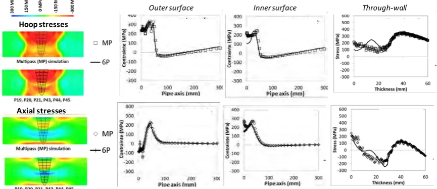
Figure 7: Comparison between the multi-pass simulation (MP) and the different simplified simulations

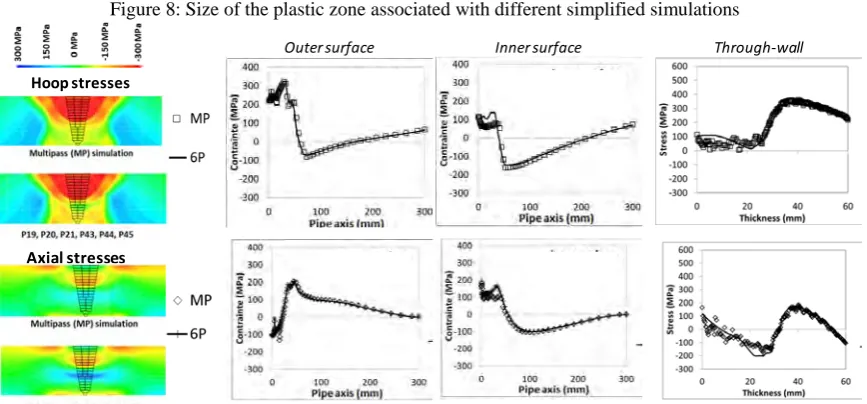
The optimal choice of the beads that should be considered for test case 3 is given in figure 8. In that case, the deposit of beads 19, 20 and 21 are simulated, assuming that passes 1 to 18 are already present in the model, but with a zero initial stress field. Following computation of pass 21, passes 22 to 42 are included in the FE model without any stress, and the deposit of beads 43, 44 and 45 are finally simulated (thermal and mechanical transient evolutions) from the stress-state resulting from the previous step (end of pass 21). With this method, numerical weld simulations are performed for only 6 passes instead of 43, allowing an noticeable time saving. In this case, the computation time is divided by 7.

Figure 8: Size of the plastic zone associated with different simplified simulations

Figure 9: Test 3A -Comparison between the multi-pass simulation (MP) and the simplified simulation

Outer surface Inner surface Through‐wall

H

o

o

p

st

re

sses

Ax

ia

l

st

re

ss

es

Hoop stresses

The final result with this simplified method is compared to the multi-pass one on figure 9 and 10. A very good agreement is obtained with the reference results, for the outer and inner residual stress profiles in both axial and hoop directions, as well as for the through-wall stress evolutions.

Figure 10: Test 3B Comparison between the multi-pass simulation (MP) and the simplified simulation

To compare the results of the different simulations, the axial and circumferential stress profiles along the outer surface, the inner surface, and through the thickness, have been considered for each test. For each profile, the average discrepancy (absolute value) over the whole profile, between the multi-pass computation and the simplified one (result difference at every calculation point), has been calculated. The correspondent discrepancies, for each profile, are summarized in table 1. Then, the average discrepancy is calculated and compared to the room temperature yield stress of the base metal (table 2). It shows that the average differences, reported to the yield stress, are less than 15% for all the cases, which is very satisfactory considering the corresponding reduction of time computation.

Table 2 gives a recap of the CPU times required for each tests. The reduction is drastic for all the tests. Though the CPU times are not very high for 2D models even for the complete multi-pass simulations, one has to consider the expected time saving for 3D simulations, for which a single pass can take more than one day of CPU time. The reduction from 43 passes to only 6 passes, as for test 3, would then be particularly attractive. This would make a multi-pass weld FE simulation on very big components within an engineering framework feasible.

Table 2: Average discrepancies in MPa between the multi-pass simulation (MP) and the simplified

simulation for test 1 to 3

Table 3: Indicative computation time for the different multi-pass and simplified simulations (test 1 to 3), for a same computer and a same number of CPU

Outer surface Inner surface Through‐wall

Hoop stresses

Test case 1

Test case 2

Test case 3

Multi-pass modeling

25 min

-

11 beads

2h30

-

23 beads

17h30

-

45 passes

Simplified method

2 min

-

1 bead

7 min

-

1bead

2h20

-

6 passes

Time ratio

/12 ~/20

~/7

METHODOLOGY RECOMMANDATION

The successive steps of the simplified method can be summarized as follows:

a) First, estimation of the plastic zone radius (PZR) corresponding to each bead of the groove. On classical configurations such as pipes or plates, this could be achieved using classical analytical formulas such as Eqn.2, knowing the thermal and mechanical parameters and heat input. For more specific geometries, this can be done numerically by running a FE simulation for a single bead, and by analyzing the corresponding PZR

b) Knowing a PZR for each layer, the selection of the retained beads is performed, chronologically from the last deposited bead of the weld sequence, to the first deposited one. Considering the last layer, all the weld passes that are present within the PZR are excluded from the analysis. Then the last deposited layer before the excluded ones is selected, and the radius of its plastic zone is evaluated. Then the selection process is repeated until the very first layer of the weld sequence is reached.

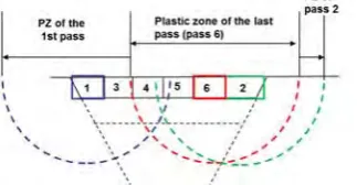
c) In every selected layer, the beads composing the layers are selected according to the same methodology as in b). If the layer contains only a few beads, only the last bead of the layer may be selected. If the layer contains more beads, they must be selected from the last deposited one, going back to the first one, according to the plastic zone’s size. As an example, figure 15 shows a specific sequence in a 6 beads layer. Only passes n°1, 2 and 6 are to be taken into account in the analysis. d) The simulation of welding of the selected beads is conducted as it is for the complete multi-pass

analysis. The unselected beads are also added in the model following the weld sequence, but with zero stress fields, allowing very fast computations.

Figure 11: Bead selection in a given layer – only beads 1, 2 and 6 can be taken in the weld analysis

The proposed simplified method is an interesting alternative to macro-bead procedures, even if the computation time is higher (Rossillon and Depradeux (2013) it does not involve any fitting of the input data. It must be emphasized that the modeling of each selected bead deposit is performed in the same manner as in the complete multi-pass analysis. So the heat input in the selected beads can be deduced directly from weld parameters, as defined previously. Therefore, this method is a also a “predictive” one (no fitting). Of course, this simplified method, suitable for weld residual stresses predictions, is not adequate for predicting the amount of cumulated plastic strains in the weld zone.

CONCLUSION

In this paper, a simplified method to compute weld residual stresses in multi-pass welds with FE method is proposed. This method consists in selecting a few appropriately selected beads, and to simulate their deposit as it is done in a complete multi-pass weld simulation, adding the other bead in the model with a zero stress state. This method allows a drastic reduction of computation times: CPU time are divided by a factor 10. This is very promising and interesting for 3D models. For the moment, this method has been well validated on different configurations of pipes girth welds, and a practical method to select the beads retained has been defined.

another paper (Rossillon and Depradeux (2013), and compared to multi-pass results and to a macro beads analysis. In parallel, further investigations of this method are being performed on a full 3D model like J welds.

ACKNOWLEDGMENTS

The authors want to acknowledge Dr. Claude Amzallag for introducing the idea of selecting an appropriately reduced number of passes.

NOMENCLATURE

PWR Pressurised Water Reactor MP Multi-pass

PZR Plastic Zone Radius E Young modulus U Tension I Intensity

 Efficiency parameter depending on the welding technology

V velocity of the welding torch S cross section of the pass

Q/V welding energy per meter units

 Thermal coefficient

y Yield stress  Density C specific heat t Pipe thickness R Pipe radius

REFERENCE

Bouchard P.J. (2007), “Validated residual stress profiles for fracture assessments of stainless steel pipe girth welds”,

International Journal of Pressure Vessels and Piping, 84, 195–222.

Brickstad B. and Josefson B. L. (1998), “A parametric study of residual stresses in multi-pass butt-welded stainless steel pipes”, International Journal of Pressure Vessels and Piping, 75, 11-25.

Deng D., Murakawa H. and Liang W. (2008), “Numerical and experimental investigations on welding residual stress in multi-pass butt-welded austenitic stainless steel pipe”, Computational Materials Science 42, 234–244. Dong P. (2007), “On the Mechanics of Residual Stresses in Girth Welds”, Journal of Pressure Vessel Technology 19,

345-353.

Lee C.H. and Chang K.H. (2008), “Three-dimensional finite element simulation of residual stresses in circumferential welds of steel pipe including pipe diameter effects”, Materials Science and Engineering A 487 210–218

Leggatt R.H. (2008), “Residual stresses in welded structures”, International Journal of Pressure Vessels and Piping,

85, 144–151.

Liu C., Zhang J.X. and Xue C.B. (2011), “Numerical investigation on residual stress distribution and evolution during multi-pass narrow gap welding of thick-walled stainless steel pipes”, Fusion Engineering and Design

86, 288–295.

Muránsky O., Smith M.C., Bendeich P.J. and Edwards L. (2011), “Validated numerical analysis of residual stresses in Safety Relief Valve (SRV) nozzle mock-ups”, Computational Materials Science 50, 2203–2215.

Ogawa K., Deng D, Kiyoshima S., Yanagida N. and Saito K. (2009) “Investigations on welding residual stresses in penetration nozzles by means of 3D thermal elastic plastic FEM and experiment”, Computational Materials Science, 45, 1031–1042.

R6 - Assessment of the integrity of structures containing defects, British Energy, 2004

Rossillon F. and Depradeux L. (2011), “A methodology for a simplified thermo-mechanical welding simulation in an engineering framework”, Proc. SMiRT 21, India Div-III ID 407

Rossillon F. and Depradeux L. (2013), “Simplified computation of the welding process on a steam-generator divider plate “,PVP2013-97238, ASME 2013 Pressure Vessels and Piping Conference, Paris, France

Stacey A., Barthelemy J.-Y., Leggatt R.H. and Ainsworth R.A. (2000), “Incorporation of residual stresses into the SINTAP defect assessment procedure”, Engineering Fracture Mechanics 67 573-611.

Smith M.C. and Smith A., C. (2009), “NeT Bead-on-plate round robin: Comparison of transient thermal predictions and measurements”, International Journal of Pressure Vessels and Piping 86, 96-109