Conversion of Evanescent into Propagating Guided Waves in Plates.

ABSTRACT

YAN, XIANG. Conversion of Evanescent into Propagating Guided Waves in Plates. (Under the direction of Dr. Fuh-Gwo Yuan).

Current guided wave-based damage detection methods using advanced signal/image processing techniques can only process the damage information contained in the propagating guided waves since evanescent guided waves scattered from the damage decay exponentially away from it. The valuable subwavelength damage information concealed in the evanescent waves is therefore permanently lost in the damage image which may prevent the detection of the damage at the very early stage. Motivated by the possibility of achieving a ‘super resolution’ damage image by re-capturing subwavelength damage information contained in evanescent guided waves, this dissertation presents a feasibility study of converting evanescent into propagating guided waves in isotropic plates so that the far-field sensors can retrieve such valuable localized (subwavelength) damage information.

The properties of evanescent and propagating guided waves, i.e., Lamb waves and shear horizontal waves (SH waves), are first investigated by revisiting the formation of guided waves in isotropic plates and are characterized by the complex-valued dispersive curves. The important phase information and mode shapes for the propagating and evanescent guided waves are uncovered.

an elastic plate can be completely described by a complex power flow, with real part representing the radiative power and imaginary part describing the reactive power. This type of separation of complex power flow is then proved to be related to the usual separation made on the basis of propagating and evanescent guided waves as propagating guided waves carry pure real power flow and the power flow for evanescent waves turns out to be pure imaginary.

The conversion of evanescent into propagating Lamb waves is substantiated by prescribing Lamb evanescent time-harmonic displacements or tractions distributed through a narrow aperture at the edge of a semi-infinite plate. First, a purely Lamb evanescent field can be generated when Lamb evanescent displacements or tractions are incident upon the entire edge of the plate. The amplitude coefficient of the propagating Lamb waves being converted from evanescent is determined through a theoretical formulation based on the complex reciprocity theorem via the finite element analysis (FEA) and is verified through the validation of a complex power conservation relation. Power conversion efficiency analysis shows that the propagating power converted from evanescent excitation is strongly frequency dependent and can be significant.

the amplitude coefficient of the converted propagating SH mode from evanescent and the amplitude coefficient is verified by proving a complex power conservation relation. Power conversion analysis shows that the conversion efficiency for propagating SH modes converted from evanescent varies dramatically as excitation frequency changes and can be significant.

Conversion of Evanescent into Propagating Guided Waves in Plates

by Xiang Yan

A dissertation submitted to the Graduate Faculty of North Carolina State University

in partial fulfillment of the requirements for the degree of

Doctor of Philosophy

Aerospace Engineering

Raleigh, North Carolina 2014

APPROVED BY:

_______________________________ ______________________________ Dr. Fuh-Gwo Yuan Dr. Guoliang Huang

Committee Chair

DEDICATION

BIOGRAPHY

Xiang Yan was born on July 27, 1986 in Guannan, Jiangsu Province, China. He graduated from Xinhai High School of Lianyungang in 2005 and in the same year, he was admitted to Jiangsu University, Zhenjiang, China, studying Civil Engineering. In 2009, he received his Bachelor degree at Jiangsu University. After graduation, he was admitted without examination to study in the Solid Mechanics PhD program and studied one-year in the same university.

In 2010, he was enrolled as a doctoral student in the Department of Mechanical and Aerospace Engineering at North Carolina State University under the direction of Dr. Fuh-Gwo Yuan. He conducted research on flexoelectric sensing and acoustic/elastic metamaterials for structural health monitoring (SHM) between 2011 and 2013. He started this fundamental dissertation work on the conversion of evanescent into propagating guided waves in plates towards the goal of achieving subwavelength damage detection and imaging for SHM in the summer of 2011 and was awarded a M.S. degree in 2012. He is being supported by the China Scholarship Council (CSC) and North Carolina State University.

ACKNOWLEDGMENTS

First and foremost, I would like to express my deepest gratitude to my advisor and committee chair, Dr. Fuh-Gwo Yuan, for the time and efforts that he spent on me in helping me pursuing my Ph.D. degree. His guidance, knowledge, patience, and enthusiastic encouragement have been an invaluable source of inspiration throughout my Ph.D. study. It is him who makes me understand there is no shortcut for research but hard working; It is him who gives me enough freedom so that I can step into new research directions; It is him who makes me realize exploring unknowns is key to research and the process for exploring is always important than the outcomes. It is my great honor, fortune, and pleasure in having the opportunity working with Dr. Yuan to develop my research base and skills and independent research ability. Thank you Dr. Yuan for his candid, pertinent, and beneficial suggestions on my career and life planning; he is not only an academic advisor, but also a mentor for life. Thank you, Dr. Yuan!

I would also like to thank all my other committee members, Dr. Guoliang Huang, Dr. Jingyan Dong, Dr. Kara Peters, and Dr. Xiaoning Jiang, who have offered me superb classes, and invaluable suggestions for my dissertation research explorations. Special thanks to Dr. Ying Luo who was my graduate academic advisor when I was in Jiangsu University, China. It was his encouragement and continuous support so that I was able to pursue my Ph.D. degree in the states.

Li, Dr. Rui Zhu, Dr. Fujun Xu, Dr. Wensong Zhou, Dr. Zhenxin Cao, Dr. Chris Page, Mr. Jiaze He, Mr. Chao Wan, Mr. Che-Yuan Chang, Mr. Ningyi Zhang, Ms. Yuling Liu, Mr. Sri Vikram Palagummi, Mr. Mohammad Harb, Mr. Tyler Hudson, Mr. Patrick Leser and Mr. Donato Girolamo. Especially thanks to Dr. Shaorui Yang, who is always ready to answer me any theoretical questions related to solid mechanics.

TABLE OF CONTENTS

LIST OF FIGURES

...

LIST OF SYMBOLS AND ABBREVIATIONS

...

Chapter 1 Introduction

...

1.1 Research Motivation ... 3

1.2 Literature Review ... 5

1.2.1 Non-Propagating (Evanescent) Waves in Plates... 5

1.2.2 Retrieving Evanescent Waves Information for Subwavelength Imaging ... 7

1.3 Objective and Outline... 11

Chapter 2 Guided Waves in Plates

...

2.1 Introduction ... 15

2.2 Bulk Waves ... 17

2.3 Lamb Waves ... 23

2.3.1 Basic Equations ... 23

2.3.2 Lamb Wave Dispersion Relation ... 28

2.3.3 Propagating and Evanescent Lamb Waves ... 29

2.4 SH Waves ... 48

2.4.1 Basic Equations and SH Waves Dispersion Relation ... 48

2.4.2 Propagating and Evanescent SH Waves ... 51

2.5 Summary ... 58

Chapter 3 Reciprocity, Orthogonality Relations and Power Flow for

Guided Waves in Plates

...

3.1 Introduction ... 60

3.3 Orthogonality Relations ... 70

3.3.1 Orthogonality Relations for Lamb Waves ... 74

3.3.2 Orthogonality Relation for SH Waves ... 76

3.4 Power Flow ... 78

3.4.1 Power Flow for Lamb Waves in Plates ... 82

3.4.2 Power Flow for SH Waves in Plates ... 86

3.5 Summary ... 90

Chapter 4 Conversion of Evanescent into Propagating Lamb Waves in

Plates

...

4.1 Introduction ... 93

4.2 Generation of Evanescent Lamb Waves ... 93

4.2.1 Through Edge Displacement Excitations... 94

4.2.1.1 Theoretical Formulation... 94

4.2.1.2 Finite Element Analysis Verification... 97

4.2.2 Through Edge Traction Excitations ... 105

4.2.2.1 Theoretical Formulation... 105

4.2.2.2 Finite Element Analysis Verification... 106

4.3 Conversion of Evanescent into Propagating Lamb Waves through Narrow Apertures 113 4.3.1 Conversion of Evanescent into Propagating Lamb Waves- Finite Element Modeling ... 118

4.3.2 Determination of Amplitude Coefficient of the Converted Propagating Lamb Waves-Theoretical Formulations ... 121

4.3.2.1 Evanescent Displacement Excitations ... 121

4.3.2.2 Evanescent Traction Excitations ... 124

4.3.3 Power Conversion Efficiency for the Propagating Lamb Waves ... 126

4.3.3.1 Verification on the Amplitude Coefficient (Am) of the Converted Propagating Lamb Waves ... 127

4.3.3.2 Propagating Power Conversion Efficiency (ξ)... 132

Chapter 5 Conversion of Evanescent into Propagating SH Waves in Plates

...

5.1 Introduction ... 145

5.2 Generation of Evanescent SH Waves... 145

5.2.1 Through Edge Displacement Excitations... 146

5.2.1.1 Theoretical Formulation... 146

5.2.1.2 Finite Element Verification... 149

5.3 Conversion of Evanescent into Propagating SH Waves through Narrow Apertures 157 5.3.1 Conversion of Evanescent SH Waves into Propagating-Finite Element Modeling ... 162

5.3.2 Determination of Amplitude Coefficient of the Converted Propagating SH Waves- Theoretical Formulations ... 165

5.3.3 Power Conversion Efficiency for Propagating SH Waves ... 169

5.3.3.1 Verification on the Amplitude Coefficient (Am) of the Converted Propagating SH Waves... 170

5.3.3.2 Propagating Power Conversion Efficiency (ξ)... 173

5.4 Summary ... 175

Chapter 6 Conclusions and Future Work

...

6.1 Conclusions and Contributions beyond Previous Work ... 180

6.2 Future Work ... 182

LIST OF FIGURES

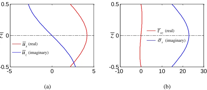
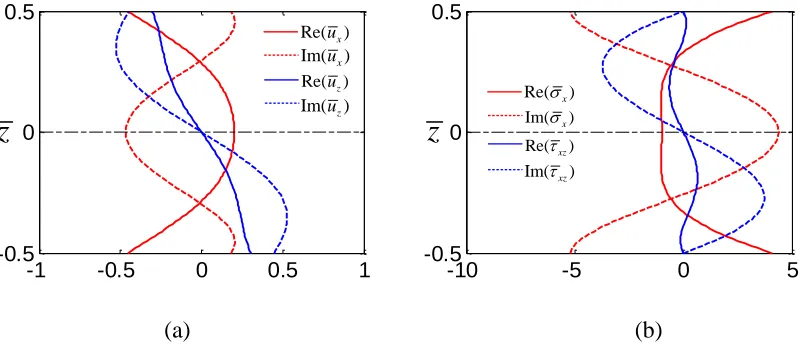
Figure 2.8 Mode shapes for A1 mode propagating Lamb waves at ωh/cT = 3.56 (fh = 1.8

MHz·mm) located in region I of Figure 2.7. (a) Displacement mode shapes; (b) Stress mode shapes. ... 43 Figure 2.9 Mode shapes for S0 mode propagating Lamb waves at ωh/cT = 3.56 (fh = 1.8

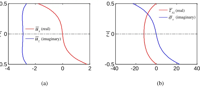
MHz·mm) located in region II of Figure 2.7. (a) Displacement mode shapes; (b) Stress mode shapes. ... 44 Figure 2.10 Mode shapes for A0 mode propagating Lamb waves at ωh/cT = 3.56 (fh = 1.8

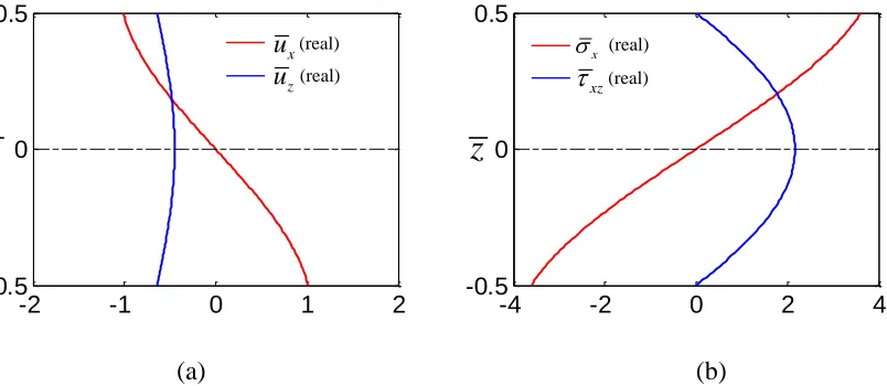
MHz·mm) located in region III of Figure 2.7. (a) Displacement mode shapes; (b) Stress mode shapes. ... 45 Figure 2.11 Mode shapes for S0 mode propagating Lamb waves at ωh/cT = 7.4 (fh = 3.74

MHz·mm) located in region III of Figure 2.7. (a) Displacement mode shapes; (b) Stress mode shapes. ... 46 Figure 2.12 Mode shapes for A1 mode evanescent Lamb waves at ωh/cT = 1.8 (fh = 0.9

MHz·mm). (a) Displacement mode shapes; (b) Stress mode shapes. ... 47 Figure 2.13 Mode shapes for S1/ S2 mode evanescent Lamb waves at ωh/cT = 1.8 (fh = 0.9

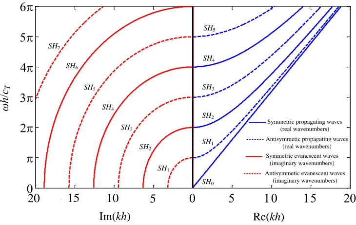
Figure 2.18 Propagating SH wave group velocity dispersive curves. ... 55 Figure 2.19 Stress mode shapes for propagating SH modes at ωh/cT = 3.972 (fh = 2

MHz·mm) (a) SH0 mode, (b) SH1 mode (The normalized stresses

are used). ... 57 Figure 2.20 Stress mode shapes for evanescent SH modes at ωh/cT = 1.986 (fh = 1 MHz·mm)

(a) SH2 mode, (b) SH1 mode (The normalized stresses are used). 57

Figure 3.1 Static reciprocity relations (Elastic body with volume V and boundary S subjected to concentrated load f1 and f2). ... 61

Figure 3.2 The domain for applying the integral form complex reciprocity relations in an elastic plate... 71 Figure 3.3 The complex power flow into the plate due to source excitation (tractions or displacements applied at the edge of the plate). ... 82 Figure 3.4 The velocity and stresses for Lamb waves at any arbitrary cross section in a plate. ... 83 Figure 3.5 The velocity and shear stresses for SH waves at any arbitrary cross section in a plate. ... 87 Figure 4.1 Schematic view of a semi-infinite plate of thickness h where Lamb evanescent displacement or traction excitations are prescribed at the edge across the thickness to generate a purely Lamb evanescent field. ... 94

/ , /

xy xy G yz yz G

   

/ , /

xy xy G yz yz G

Figure 4.2 Time-harmonic normalized displacement distributions applied at x = 0 for the generation of (a) A1 evanescent mode; (b) S1/S2 evanescent mode; (c) A2/A3 evanescent mode

at ωh/cT = 0.0946 (fh = 0.3 MHz·mm). ... 98

Figure 4.3 Evanescent Lamb wave displacement field generated by edge displacement excitations at ωh/cT = 0.0946 (fh = 0.3 MHz·mm) (a) A1 evanescent mode; (b) S1/S2

evanescent mode; (c) A2/A3 evanescent mode. ... 102

Figure 4.4 Time-harmonic normalized traction distribution at x = 0 for the generation of (a) A1 evanescent mode; (b) S1/S2 evanescent mode; (c) A2/A3 evanescent mode at ωh/cT =

0.0946 (fh = 0.3 MHz·mm). ... 107 Figure 4.5 Evanescent Lamb wave displacement field generated by edge traction excitations at ωh/cT = 0.0946 (fh = 0.3 MHz·mm), (a) A1 evanescent mode; (b) S1/S2 evanescent mode;

(c) A2/A3 evanescent mode. ... 110

Figure 4.6 Cross section of a semi-infinite plate for studying conversion of evanescent waves into propagating. The plate (thickness = h) is subject to evanescent excitations at the left boundary through a small aperture (height = h1). (a) Symmetric aperture with respect to x

axis, (b) asymmetric aperture with respect to x axis. ... 115 Figure. 4.7 (a) Complex dispersion curves and (b) group velocity dispersive curves used for studying converting evanescent into propagating Lamb waves. (The green solid dot denotes the A1 evanescent mode excited at ωh1/cT and the red solid dots represent possible

Figure 4.9 Conversion of A1 evanescent Lamb wave into A0 propagating mode through a

narrow aperture (h1 = 3mm, h = 6mm). Excitation frequency f = 100 kHz. (a) Total

displacement field- under displacement excitations, (b) total displacement field- under traction excitations. ... 120 Figure 4.10 Representation of stresses and displacements in the aperture due to evanescent Lamb mode exciation and at any arbitrary far-field section of the plate for the calculation of power delivered to the plate and power flow outward by propagating Lamb modes. ... 127 Figure 4.11 Comparison of the real part of the complex power into the plate through a symmetric aperture (h1 = 3mm and h = 6mm) and the real power flow for converted

propagating Lamb waves, (a) A1 evanescent displacement excitations and (b) A1 evanescent

traction excitations. (Log power is used in the plots). ... 130 Figure 4.12 Complex power flow input through a symmetric aperture (h1 = 3mm and h =

6mm) as a function of normalized frequency under (a) A1 evanescent displacement excitation,

(b) A1 evanescent traction excitation. (The complex power is in log scale). ... 134

Figure 4.13 Propagating power efficiency of converting evanescent A1 Lamb wave into

propagating Lamb waves as a function of frequency. The plate is excited by the (a) evanescent A1 displacement distribution, (b) evanescent A1 traction distribution at the left

edge through a symmetric aperture. ... 136 Figure 4.14 Propagating power efficiency of converting evanescent A1 Lamb wave into

propagating as a function of frequency. The plate is excited by the (a) evanescent A1

Figure 5.1 Schematic view of a semi-infinite plate of thickness h where evanescent displacement is applied at the edge across the thickness to generate a purely SH evanescent field. ... 146 Figure 5.2 Schematic of a semi-infinite plate with extra absorbing region for the generation of pure evanescent SH waves. ... 153 Figure 5.3 Time-harmonic displacement distribution applied at x = 0 for the generation of (a) SH1 evanescent mode; (b) SH2 evanescent mode at ωh/cT = 0.5944 (fh = 0.3 MHz·mm). ... 154

Figure 5.4 SH evanescent displacement field in the antiplane direction generated by edge displacement excitations at ωh/cT = 0.5944 (fh = 0.3 MHz·mm) (a) SH1 evanescent mode; (b)

SH2 evanescent mode. ... 156

Figure. 5.5 (a) Complex dispersion curves and (b) group velocity dispersive curves used for the study of converting evanescent into propagating SH waves. (The green solid dot denotes the SH1 evanescent mode excited at ωh1/cT and the pink solid dots represents possible

propagating SH modes that can be converted depends on the frequency ωh/cT). ... 159

Figure 5.7 Cross section of a semi-infinite plate for studying conversion of evanescent SH waves into propagating. The plate (thickness = h) is subject to evanescent displacement. .. 161 Figure 5.8 Schematic of a semi-infinite plate using an absorbing region adjacent to the main plate to study the conversion of evanescent into propagating SH waves by prescribing evanescent displacement distributions through a symmetric aperture (h1) at the edge of the

conversion at 300 kHz (ωh/cT = 3.566) ; (c) SH1 mode conversion at 400 kHz (ωh/cT =

4.7547). ... 164 Figure 5.10 Representation of stresses and displacements in the aperture due to evanescent SH mode excitation and at any arbitrary far-field section of the plate for the calculation of power delivered to the plate and power flow outward by propagating SH modes. ... 169 Figure 5.11 Complex power flow delivered into a symmetric aperture (h1 = 3mm and h =

6mm) under SH1 evanescent displacement excitation as a function of normalized frequency.

(The complex power is in log scale). ... 172 Figure 5.12 Comparison of the real part of the complex power input to the plate through a symmetric aperture under SH1 evanescent displacement excitation and the real power flow

for the converted propagating SH modes. (Log power is used in the plots). ... 173 Figure 5.13 Power conversion efficiency of converting evanescent SH1 mode into

propagating SH1 mode as a function of normalized frequency. The plate is excited by

evanescent SH1 displacement at the left edge through a symmetric aperture. ... 177

Figure 5.14 Power conversion efficiency of converting evanescent SH1 mode into

LIST OF SYMBOLS AND ABBREVIATIONS

Coordinate Systems and Locations

x = (x1, x2, x3) = (x, y, z) Rectangular coordinate system variables

Greek Symbols

ξ Power conversion efficiency

λ Wave length

μ Shear modulus

ν Poisson’s ratio

ω Angular frequency

c Cut-off angular frequency

ρ Density

 Scalar potential

 Vector potential

θ Phase surface

σ Stress tensor Roman Symbols

A Amplitude coefficient

cg Group velocity

cL Longitudinal velocity

cT Transverse velocity

E Young’s modulus

f Body force f Frequency h Plate thickness

Im Imaginary part of complex variables

k Wavenumber

L Length of the plate

n Surface normal unit vector

P Complex acoustic Poynting vector

PC Complex power flow

Re Real part of complex variables

S Strain tensor

s Compliance tensor

T Traction vector

u Displacement vector

v Velocity vector

PW Propagating waves

Modifiers

* Complex conjugate

 Del operator

If we knew what it was we were doing, it would not be called research, would it?

Chapter 1

1.1

Research Motivation

in

u

damage

propagating wave

evanescent wave

Distributed sensors

actuator

scatter

u

Figure 1.1 A schematic of common guided wave based SHM set up for damage detection using omnidirectional circular piezoelectric wafers.

As plate-like structures are often seen in a number of mechanical, aerospace and civil applications, detecting the damage at an early stage is critical for safe operation of these structures. A ‘super-resolved’ image can provide much more details about the damages so that they can be diagnosed at the incipient state. Motivated by the possibility of achieving a ‘super resolution’ damage image by re-attaining subwavelength damage information concealed in the evanescent waves, the goal of the dissertation work is to investigate the feasibility of converting evanescent into propagating guided waves in plate-like structures so that the sensors located in the far-field can retrieve such valuable localized (subwavelength) damage information. The work presented in this dissertation provides a theoretical foundation for the study of converting evanescent into propagating guided waves (including both Lamb waves and SH waves) in plates and may holds promise for the subwavelength damage imaging for plate-like structures.

1.2

Literature Review

1.2.1 Non-Propagating (Evanescent) Waves in Plates

antisymmetric Lamb modes (real roots for Rayleigh Lamb equation). Following Lamb in the next half century, most of the efforts had been attempted on the characterization of higher order modes of propagating waves. It was not until (1955), the purely imaginary roots of the dispersion equation were obtained by Lyon. The presence of complex roots of the dispersion equation was demonstrated in the remarkable work done by Mindlin (1957). Shortly after that, a complete dispersion curves including real, imaginary, and complex wavenumbers is elaborated by Mindlin (1960). The amplitudes of Lamb waves with purely imaginary or complex wavenumbers exponentially decay away from the source, and these waves are usually referred to as non-propagating or evanescent Lamb waves. The propagation of SH waves is much simpler, since they are decoupled from the L-SV (Lamb) waves and have simple dispersion characteristics. A complete dispersion curves including pure imaginary and real wavenumbers of SH waves in plates can be found in many books (Achenbach, 1975; Graff, 1975; Miklowitz, 1978; Auld, 1990). The SH waves with pure imaginary wavenumbers which exhibit exponentially decay and thus are called non-propagating or evanescent SH waves.

Torvik (1967) is highly recommended. The purpose of studying these localized modes is to obtain an accurate field distribution around the structural discontinuities when applying normal mode superstition techniques (e.g., Auld, 1976; Gunawan et al., 2004, Moreau, 2006). In addition, as guided waves are scattered from damage/cracks (scatters), the superposition of incident and scattered guided waves needs to satisfy the boundary condition on the top and bottom of the plate as well as the surface of the scatter. The existence of non-propagating modes (evanescent waves) in the scattered waves is a necessary condition to fulfill this requirement (Simonetti et al., 2005; An et al., 2013). After considering the non-propagating modes, a complete description of wave fields around the scatters can be obtained. Apart from the research related to the evanescent guided waves mentioned above, as far as we know, very few works (Diligent et al., 2003, Predoi, 2004; Simonetti et al., 2005) in the literature solely dedicated to study the property or gave some insights on the physical meaning of evanescent guided waves.

1.2.2 Retrieving Evanescent Waves Information for Subwavelength Imaging

wavelength of the surface of the specimen. It was not until (1972) Ash and Nicholls experimentally proved Synge’s idea. In their experiment, two ‘object’ separated by λ/60 which broke the diffraction limit in the microwave regime. Since then this near-field scanning technique became the well-established field called ‘Near-field Scanning Optical Microscopy’ (NSOM) (Betzig et al., 1991; Lewis et al., 2001; Courjon, 2003) and has been widely used. Generally, there are three approaches (Courjon, 2003) that are available in NSOM: illumination mode, collection mode and apertureless mode. The physics behind all of the three approaches is that the evanescent waves produced at the surface of the specimen are converted to propagating waves due to the tunneling effect. With the converted propagating waves from evanescent, the localized information about the specimen is recovered and enables the realization of subwavelength resolution. Since NSOM uses point-by-point scanning, the collected signals still need to be post-processed in order to be imaged and thus it is time-consuming.

negative permeability μ) and acoustic fields (e.g., Ambati et al., 2007; Jia et al., 2010; Park et al., 2011) (negative density ρ and/or negative modulus E). The amplification of evanescent waves relies on the fact the NIM supports resonant surface waves in which evanescent waves can be effectively coupled into these surface modes and enhanced by their resonant nature when their wave vectors are matched (Zhang et al., 2008). As the resonance based NIM ‘superlenses’ is constructed using realistic materials, the intrinsic energy dissipation or loss hinders the resolution of a ‘perfect image’. Another drawback of ‘superlenses’ is that the distance between the slab and both the image and object, as well as the thickness of the slab is strictly restricted so as to obtain an efficient resonant enhancement of evanescent waves. Another type of superlens using photonic crystals (e.g. Luo et al., 2003) and phononic crystals (Sukhovich et al., 2009) which can exhibit negative refraction were proposed for subwavelength imaging. The coupling between incident evanescent waves and the slab mode of photonic crystals or phononic crystals leads to the amplification of evanescent waves. Those superlenses are only capable of projecting subwavelength image in the near field, as the evanescent waves will decay again away from the lenses.

Salandrino (2006) independently proposed that a cylindrical geometry anisotropic metamaterials with hyperbolic dispersion, termed as ‘hyperlens’, can allow image magnification for subwavelength imaging. When evanescent waves enter the anisotropic medium, the evanescent waves become propagating and can propagate through the hyperlens. The working mechanism (Lu et al., 2012) is essentially because the anisotropic medium with hyperbolic dispersion relation continuously compresses the large wave vectors of the original evanescent wave vectors in the hyperlens region. Since the transverse wave vectors are compressed to be sufficiently small, the propagating waves remain propagating as they propagate outside the anisotropic region and can propagate to the far-field. The concept of hyperlens and subwavelength imaging were successfully verified by experiments in the electromagnetic (e.g., Lee et al., 2007; Liu et al., 2007) and acoustic fields (e.g., Ao et al., 2008; Torrent et al., 2008; Li et al., 2009). Among these work, Lee (2011) proposed an elastic hyperlens using a near flat dispersion relation that can resolve two sources in a plate which is 0.45λ apart.

interaction between the scatters that cause the evanescent waves to be encoded. Since the higher order effects in the scattering fields are difficult to be described, in other words, not all the evanescent modes can be encoded, this prevents a better subwavelength image to be obtained.

1.3

Objective and Outline

In view of the motivation and the literature review for the dissertation, conversion of evanescent into propagating guided waves in plates is probably the best way to achieve far-field subwavelength damage detection and imaging in plates. As the study on conversion of evanescent into propagating guided waves in plates is absent in literature, the objective of the dissertation is to give a comprehensive study on the evanescent guided waves and quantitatively investigate the conversion process for converting evanescent into propagating guided waves in isotropic plates:

 To characterize the properties of evanescent guided waves in isotropic plates;

 To separate the complex power flow into the plate on the basis of propagating and evanescent guided waves.

 To provide analytical model for the generation of evanescent guided waves in isotropic plates and verify using FEA.

This study would provide a theoretical foundation for the future study of far-field subwavelength damage detection and imaging in plates.

In order to explore the feasibility of converting evanescent into propagating guided waves in plates, this dissertation is organized as follows:

Chapter 1 presents the motivation and problem statement, the literature review, objective and outlines of the dissertation work.

Chapter 2 introduces a complete theoretical description of guided waves propagation in plates. The bulk wave propagation in an infinite medium is first studied followed by the study of the two types of guided waves in plates: Lamb waves and SH waves. The properties of propagating and evanescent guided Lamb and SH waves are studied, respectively. The propagating and evanescent guided waves are first characterized from the complex dispersion curves. The phase information of propagating and evanescent guided waves is then investigated from the displacements and stresses distributions.

Chapter 3 describes the reciprocity, orthogonality relations and power flow for guided waves in plates. The generic reciprocity relation is first derived and is discussed for Lamb and SH waves, respectively. The orthogonality relations for Lamb waves and SH waves are then derived from the reciprocity relations. Finally, the power flows for propagating and evanescent guided waves in plates are discussed in detail.

evanescent displacement or tractions at the edge of a 2-D isotropic semi-infinite plate. A theoretical model based on the reciprocity theorem with the aid of finite element analysis (FEA) model is then used to investigate the conversion of evanescent into propagating Lamb waves. The conversion process is studied by imposing evanescent excitations through a narrow aperture at the edge of the 2-D isotropic semi-infinite plate. The amplitude coefficient of the converted propagating waves is determined from the theoretical model with the aid of FEA is validated by proving a complex power conservation relation. Finally, the propagating power conversion efficiency for Lamb waves is studied.

Chapter 5 quantitatively investigates the conversion process of evanescent into propagating SH waves. To model the SH waves propagation in two-dimensional, the commercially available software COMSOL is proposed to solve the governing equation for SH waves in plates by a finite element method. The generation of evanescent SH waves is demonstrated by prescribing evanescent SH displacement at the edge of a 2-D isotropic semi-infinite plate and the conversion process is studied by prescribing evanescent SH displacement through a narrow aperture at the edge. The amplitude coefficient of the converted propagating mode is determined from a theoretical model based on the complex reciprocity theorem via FEA and is verified by a complex power conservation. Finally, the propagating power conversion efficiency for SH waves is defined.

Chapter 2

2.1

Introduction

The sensors are used to receive wave signals from the actuators from which the wave disturbance is generated. Such signals are then analyzed to extract information of the medium through which the wave propagates and reflected or scattered from the damages. It is therefore necessary that some background in different types of waves for different media must be acquired for complete understanding of various signal processing techniques.

If an elastic medium is under the action of an excitation varying in time, different types of traveling waves can arise in the medium. Each type of wave can transfer disturbances from one part of the medium to the other at a finite speed. The theory of stress waves of elastic media shows that in an infinite isotropic elastic solid an arbitrary disturbance is propagated by means of two types of bulk waves (Achenbach, 1975), longitudinal (P) and transverse, or shear (S), waves, each traveling with its own constant velocity. The transverse waves can be further classified as shear vertical (SV) and shear horizontal (SH) waves. Conventional ultrasonic nondestructive methods based on these waves have been used to inspect flaws with some success (Krautkramer et al., 1990 and Bray et al., 1992). Most inspection techniques, such as conventional ultrasonics or eddy currents, require a transducer to be scanned over each point of the structure which is to be inspected. This is a time-consuming process and cannot inspect in inaccessible areas.

surfaces alternately and the resulting disturbance propagation from their mutual interference is guided by the plate surfaces and is directed along the plate. The plate-like structures can serve as waveguides. The guided wave can be modeled by imposing surface boundary conditions on the equations of motion and can effectively describe the wave behavior. However, this approach introduces dispersion phenomenon; that is, the velocity of propagation of a disturbance along the plate being a function of frequency or, equivalently, wavelength. Therefore the dispersion in the case of an elastic medium is simply an interference phenomenon, rather than a physical property of the material. Consequently, the shape of the signal of a wave packet (a short-time wave train) may vary with the distance and time of propagation.

being used by exciting ultrasonic signals from smart materials mounted on or embedded in the structure for detecting localized damage in plate-like structures. The development of diagnostic techniques require the study of complicated wave propagation phenomena and relies strongly on the use of predictive modeling tools to enable the best structural health monitoring strategies to be identified and their sensitivities to be evaluated.

In this Chapter, the wave propagation in an infinite elastic medium is first studied. Two bulk wave speeds are defined and three types of waves are identified. Then two types of guided waves, Lamb waves and shear horizontal waves, are discussed. The wave solutions satisfy the equations of motions and boundary conditions related to traction-free surfaces of the two parallel flat surfaces. The concept of a dispersion relation, giving as a function k will be introduced. Since the propagating and non-propagating (evanescent) guided waves exhibit different behaviors, the properties of propagating and evanescent guided Lamb waves and SH waves are studied, respectively. The propagating and evanescent guided waves are first characterized from the complex dispersion curves. The phase information for propagating and evanescent guided waves is then investigated from the displacements and stresses distributions.

2.2

Bulk Waves

 2u+( + )u=u (2.1) where u= ( u1, u2 , u3 ) is the displacement in the medium at pointx ( x1, x2, x3 ) and time t,

is the density, and are the Lame’s constant and shear modulus, respectively. In the Helmholtz decomposition, the displacement vector is expressed by the sum of a scalar potential and a vector potential 

 u     (2.2)

Note that Eq. (2.2) relates three components of the displacement vector to four other functions: the scalar potential and the three components of the vector potential. This indicates that and the components of should be under an additional constraint condition. The condition 0 can provide the sufficient additional condition to uniquely determine the three components of u from the four components of and , but it is not a necessary condition. Some other relation between and must be specified if 0 is not used. Substituting Eq. (2.2) into (2.1) yields

2

[ ] (+ + ) [ ]= [ ]

                (2.3)

Since and 0 , the above equation upon rearranging terms leads to

2 2

[( 2 )  ] [  ] 0

          (2.4)

Clearly the equation of motion is satisfied if the potentials displacement potentials and satisfy the uncoupled wave equations

2

2_ 1  

and

2 2

2 2

1

0

T

c t



  

 

 (2.5b)

where c_L  (



 





 

 

 





 





The scalar potential represents longitudinal waves traveling with a wave speed cLwhile

the vector potential denotes transverse waves traveling with a wave speed cT. Since Eq.

(2.5) are simpler in form than the displacements equations of motion, elastic wave propagation problems in isotropic solids are usually approached by first expressing the displacement field in terms of these two potentials.

Both longitudinal and transverse waves are referred to as bulk waves since they propagate in the volume (bulk) of a solid. With the identity  () 0 and 0, the longitudinal (L) bulk waves are also called P-waves, pressure waves, compressional waves, dilatational waves, or irrotational waves. Transverse waves are often called shear (S) waves, distortional waves, equivoluminal waves, or rotational waves.

The stress wave field at large distances (compared to the dominant wavelength or smallest characteristic dimension in the medium) from an excitation source can, for many purposes, be quite accurately represented by a plane wave in a Cartesian coordinate system

ˆ

( _p )

f  / c t

u=a k x (2.6) where a is defined by the vector of the direction of motion (displacement) and kˆ is the unit vector (direction cosines) of the direction of wave propagation k, k k kˆ , k k| respectively, k is often called wavenumber, kwavevector.

It is worth noting that k xˆ constant describes a plane normal to the unit propagation wave vector kˆ and the constant represents the distance of the plane from the origin (along the normal). If the position of the plane is associated with t = 0, then for t > 0, the plane moves with speed cpin the direction of kˆ . Hence the equation of the plane at time t is

described by ˆk x - c t_p constant, which is called a wavefront. Since at any instant of time the wave crests lie in parallel planes, the motion represented by Eq. (2.6) is called a train of plane waves. Substituting Eq. (2.6) into Eq. (2.1) yields

 [a+( + )(k a )kcp2a]f''(k xˆ /cpt =) 0

Or

 [  c2p]a(  )(k a kˆ )ˆ=0 (2.7)

Since kˆ and aare two different vectors, Eq. (2.7) can be satisfied in two ways only

Eq. (2.7) yields

( 2 ) /

p L

c c     (2.9) In this case, the time-varying displacement is parallel to the direction of propagation and the wave is therefore called bulk longitudinal wave.

(b)a•kˆ 0

/

p T

c c    (2.10) In this case, the time-varying displacement is normal to the direction of propagation and the wave is therefore called bulk transverse (shear) wave. The displacement can have any direction in a plane normal to the direction of propagation. When the (x1, x2)-plane is

normally chosen to contain the vectorkˆ , motions can be either in the (x1, x2)-plane or normal

to the (x1, x2)-plane, i.e., along the x3 direction. These transverse motions propagating at the

same speed are called shear vertical (SV) and shear horizontal (SH) polarized waves, respectively. Note that to describe each type of waves, two constants (such as amplitude and phase) are needed to specify each wave type, in addition to the direction of propagation. Harmonic waves are steady-state waves; waves which are not steady-state are said to be transient waves (pulses). However, the transient waves in linear elastic materials can be obtained by superimposing harmonic waves in Fourier integrals. A plane harmonic wave propagating with phase velocity cpin a direction of wave vector kˆ is often convenient to

represent the wave in a complex form

ˆ

[ ( / p )] [( / p )]

i c t i c t

e    e  

 k x  k x

where ais a complex vector consisting of amplitude and phase angle, and cp/ k . is the

angular (circular) frequency (radians per second) and k is the wavenumber.

In all linear operations on the complex wave form Eq. (2.11), the real part of the derived wave solutions is equal to the solutions of the same operations applied to the real part of the original wave form. The actual solution of Eq. (2.11) is

 





Re i cp t cos[( ], arg

Re u  a e k x   a k x  t  a (2.12) The quantity

( ,t) t

 x   k x  (2.13) gives the relationship between x and t, and is generally called the phase of the waves; it determines the position on the cycle between a crest, where u is maximum, and a trough, where u is a minimum. In this phase wave equation, phase surfaces = constant are parallel planes. Hence, Eq. (2.12) represents a plane wave whose planes of constant phases are normal to the k. The gradient of -in space is the wavenumber k, whose direction is normal to the planes and whose magnitude is the average number of crests per 2units of distance in that direction. Similarly, t is the frequency , the average number of crests per 2units of

time.

,

t

 _{ }

 

 

x k  (2.14)

is the -gradient in space can also be called spatial frequency which is analogy to the frequency which is the -gradient in time.

The wave motion is recognized from Eq. (2.12). Any particular phase surface is moving with normal velocity /k in the direction of k. To emphasize the direction of the phase velocity, a phase velocity vector can be defined as

ˆ

p k



 k

c (2.15)

In terms of potentials, the harmonic wave solutions can be represented by

( )

i t

Ae 

_ k x 

(2.16)

( )

i t e  

 x

B

  _(2.17) where A and B are arbitrarily complex constants; kand are wave vectors; k k|, , cL

/ k, cT/.

2.3

Lamb Waves

2.3.1 Basic Equations

For a plate bounded by the surfaces z = h/2 and is of infinite extent in the xand y directions (x = (x, y, z) is equivalent to x = (x1, x2, x3)), the harmonic wave motion can be

A shear horizontal (SH) wave can propagate alone in the ydirection and its polarization is unchanged on reflection or refraction. This is not the case for a longitudinal (L) or shear vertical (SV) wave – these waves are coupled at a surface. Thus, reflection at a free surface is associated with partial conversion, so that an incident L (SV) wave gives a reflected L (SV) wave and a converted SV (L) wave (Figure 2.1). The wave vectors of the SV and L partial waves must all have the same components k along the x direction, and the S and L partial waves consequently propagate at different angles to the x direction for these modes, which are called Lamb waves. The analysis of wave propagation in a plate is thus more complicated for the polarized wave than for a SH wave.

Plate

x

h Lamb Wave

Incident and reflected pressure wave

Incident and reflected shear vertical wave z

P wave

S wave

Figure 2.1 Lamb wave formation in an isotropic plate with free boundaries- pressure wave and shear vertical wave incident and reflection.

wave in the xdirection. Using the Helmholtz decomposition in plane strain in the ydirection (u2 =0, () / x₂ 0), the displacement can be written as

x z u x z u z x                 (2.18)

where the subscript 2 from the function 2 has been omitted for simplicity.

The in-plane stress components can be expressed by the potentials from Hooke’s law as

2 2 2 2

2 2 2

2 2

x z x

x

u u u

x z x x z x x z

   

 _  _  _  _ _   _

       

  _{   } (2.19a)

2 2 2 2

2 2 2

2 2

x z z

z

u u u

x z z x z z x z

   

 _  _  _  _ _   _

       

  _{   } (2.19b)

2 2 2

2 2

2

z x

xz

u u

x z x z x z

  

 _  __    _

     

  _{ } (2.19c)

As discussed before, the potentials and satisfy wave equations

2 2 2

2 2 2 2

2 2 2

2 2 2 2

1

1

L

T

x z c t

x z c t

               _ _     (2.20)

The wave solution can be considered in the following complex form

( )

( )

( )

( )

i kx t i kx t z e z e        

These functions represent waves traveling coherently in the x1 direction with the same

angular frequency and the same wavenumber k. Substituting Eq. (2.21) into (2.20) leads to

1 2

1 2

( ) sin( ) cos( ) ( ) sin( ) cos( )

z A pz A pz

z B qz B qz

  

   (2.22) where

2 2

2 2 2 2

2 , and 2

L T

p k q k

c c

 

    (2.23)

p and q stands for the transverse wavenumber of the bulk pressure and shear wave, respectively. Inspection of the displacements from Eq. (2.18) by using Eq. (2.21) and (2.22) indicates the motion can be separated into symmetric and antisymmetric modes

(a) Symmetric modes, in which the longitudinal component is an even function of z and the transverse component is an odd function of z.

u

_x

u

z

x

z

(a) (b)

Figure 2.2 Lamb waves. (a) Symmetric–the longitudinal displacement is symmetric and the transverse displacement is antisymmetric with respect to the mid-plane of the plate

are opposite. (b) Antisymmetric–the transverse displacement is symmetric and the longitudinal displacement is antisymmetric with respect to the mid-plane of the plate.

The displacements associated with symmetric and antisymmetric Lamb waves are shown in Figure 2.2. The functions associated with the symmetric and antisymmetric modes are listed in the following

(a) Symmetric modes

2 1

2 1

2 1

2 2 2

2 1

2 2

2 1

2 2

2 1

cos( ) sin( )

cos( ) cos( ) sin( ) sin( )

[(2 ) cos( ) 2 cos( )]

[( ) cos( ) 2 cos( )]

[ 2 sin( ) ( ) sin( )]

x z x z xz

A pz

B qz

u ikA pz qB qz

u pA pz ikB qz

p k q A pz ikqB qz

k q A pz ikqB qz

ikpA pz k q B qz

 

 

 

   

 

  

   

  

   

(b) Antisymmetric modes

1 2

1 2

1 2

2 2 2

1 2 2 2 1 2 2 2 1 1 sin( ) cos( )

sin( ) sin( ) cos( ) cos( )

[(2 ) sin( ) 2 sin( )]

[( ) sin( ) 2 sin( )] [2 cos( ) ( ) cos( )]

x z x z xz A pz B qz

u ikA pz qB qz

u pA pz ikB qz

p k q A pz ikqB qz

k q A pz ikqB qz

ikpA pz k q B qz

                        (2.25)

where the term exp[i(kx-t)] has been dropped in the expression of displacements and stresses.

2.3.2 Lamb Wave Dispersion Relation

The dispersion relation can be obtained by imposing the traction-free boundary conditions at z = h/2

0

z xz

   (2.26) Substituting Eq. (2.26) into symmetric and antisymmetric modes in Eq. (2.24) and (2.25) gives two homogeneous equations for coefficients A and B. A necessary and sufficient condition for the existence of a solution to these equations is that the determinant of the coefficients is zero. The implicit equation between k and formed by setting the determinant to zero is usually called as dispersion relation. The dispersion relation for symmetric modes are given by

2 2 2 2

2

2 2 2

tan( / 2) 4

tan( / 2) ( )

qh k pq

ph   q k (2.27b) For antisymmetric modes

(k2q2 2) sin(ph/ 2) cos(qh/ 2)4k pq2 cos(ph/ 2)sin(qh/ 2)0 (2.28a) or

2 2 2

2

tan( / 2) ( )

tan( / 2) 4

qh q k

ph k pq



  (2.28b)

The above two equations can be combined into one equation 4

2 2 4

tan( / 2 )

4 1

tan( / 2 ) T

p ph

k q

c q qh

 



  

 _  _



  (2.29)

where γ = 0 and π/2 represent symmetric and antisymmetric Lamb wave modes, respectively. Eq. (2.29) is commonly known as Rayleigh-Lamb dispersion relation. The dispersion relation results in an infinite number of wave modes and Lamb waves dispersion curves will be plotted in next section.

2.3.3 Propagating and Evanescent Lamb Waves

The displacements for Lamb wave modes can be readily derived from Section 2.3.1 as

( )

( )

u



AU z e

( )

( )

u



AW z e

2 2 2

2 cos( / 2 )

( ) cos( ) cos( )

cos( / 2 )

k qh

U z q pz qz

k q ph

 _{ }



  

 _    _

 

2 2

2 cos( / 2 )

( ) sin( ) sin( )

cos( / 2 )

pq qh

W z ik pz qz

k q ph

 _{ }



  

  _    _

 

  (2.31b)

The stress components can be obtained as

( )

( )

At z e





_

(2.32a)

( )

( )

At z e





_

(2.32b)





At

( )

z e

2 2 2

2 2

2 cos( / 2 )

( ) 2 cos( ) cos( )

cos( / 2 ) x

p q k qh

t z i kq pz qz

k q ph

           _    _  

  (2.33a)

cos( / 2 )

( ) 2 cos( ) cos( )

cos( / 2 ) z

qh

t z i kq pz qz

ph          _    _ 

  (2.33b)

2

2 2 2 2

4 cos( / 2 )

( ) sin( ) ( )sin( )

cos( / 2 ) xz

k pq qh

t z pz k q qz

k q ph

         _     _  

  (2.33c)

4 2 2 tan( / 2 )

4 1

tan( / 2 )

p ph

k q

q qh

 



  

 _  _



  (2.34) where the non-dimensional variables are defined by

2 2 2 2 2 2 2 2 2

/ T, , ( ) , ( )

h c k kh p ph k q qh k

 _{   }  _{  } _





































Im(

kh

) Re(

kh

)



h

/c

T

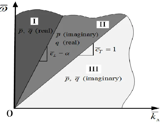
 = 0.33

A0 S0 S1 S2 A3 A1 A2 S4 A1

S1, S2

A2, A3

S3, S4

A4 S5 A2 S4 Propagating waves (Real wavenumbers) Evanescent waves (Imaginary wavenumbers) Evanescent waves (Complex wavenumbers)

15 10 5

0 2 4 6 8 10 12 14 A4 0 π/2 π 3π/2 2π 3π 5π/2 7π/2 4π 9π/2 5π

5 10 15

Im(kh) Re(kh)

ω

h

/

cT

0

ν = 0.33

0 2 4 6 8 10 12 14 16 18 20 0

0.5 1 1.5 2 2.5 3 3.5 4 4.5 5

 = 0.33

ωh/cT

cp

/

cT

A0

S0

S1

A1 S2 A3 S4 A2 A5 S3

Symmetric modes Antisymmetric modes

0 2 4 6 8 10 12 14 16 18 20 -1

-0.5 0 0.5 1 1.5 2

 = 0.33

ωh

/

c

c

/

c

Symmetric modes Antisymmetric modes

A1 A3 A2 A5

S0

A0

S1

S2

S4

S3

Figure 2.5 Lamb waves group velocity dispersive curves for propagating wave modes with Poisson’s ratio 0.33.

From the complex dispersion curve, the wavenumber k may be real, pure imaginary or complex values.

Case 1: k is pure real

From Eq. (2.30), the displacements for Lamb waves can be rewritten as i kx( t)

A e 



u U ,

where u=(ux, uz) and U=( ( ),U z W z( )). When k is pure real, the displacements are sinusoidal

propagating Lamb waves. From Figure 2.3, at any given frequency, there is a finite number of propagating Lamb modes.

Case 2: k is pure imaginary and k ≡ ikI (kI > 0)

I k x i t

A e e



u U (2.36) It is seen from Eq. (2.36), the displacements exhibit exponentially decay from positive x direction and the values of the wavenumbers determine the decay rate. The Lamb wave modes with pure imaginary wavenumbers are non-propagating (evanescent) Lamb waves. From Figure 2.3, at any given frequency, there is a finite number evanescent Lamb wave modes with pure imaginary wavenumbers.

Case 3: k is complex and k ≡ kR + ikI (kI > 0)

( )

I R k x i k x t

A e e 



u U (2.37) Eq. (2.37) can be characterized as waves propagating with a sinusoidal variation described by the real part of the wavenumbers, modulated by an exponential decaying function controlled by the imaginary part of the wavenumbers. Therefore, the Lamb wave modes with complex wavenumbers are non-propagating (evanescent) Lamb waves as well. From Figure 2.3, at any given frequency, there are an infinite number of evanescent Lamb modes with complex wavenumbers. The non-propagating A1 mode has the purely imaginary wavenumber which

means that below the A1 cutoff, the mode is characterized by the exponential decay. In

addition, among all the non-propagating modes, the magnitude of the A1 imaginary part is

From the dispersion curves, the Lamb waves are labeled as S0, S1, S2… for symmetric

modes and A0, A1, A2… for antisymmetric modes. The transition frequency that connects

propagating and evanescent Lamb modes are called a cut-off frequency. The cut-off frequency is associated with the lowest frequency at which propagating modes can exist in a mode; that is, the lowest frequency at which a given mode exist with a real-valued wavenumber. Below the cut-off frequencies, the Lamb modes are evanescent and thus evanescent fields are exponentially decaying fields that do not possess real power. The exponential decay associated with the mode is not associated with losses in the medium. Rather, the energy in the mode is stored in a region rather than being propagated freely. The power for propagating and evanescent Lamb waves in plates will be discussed in detail in the next Chapter.

Among all the Lamb wave modes, there exist two modes S0 and A0 that do not have a

cut-off frequency. For these fundamental modes, ω approaches zero as k approaches zero, and the waves are all propagating across the entire frequency range. For Lamb waves with cut-off frequencies, the cut-off frequency ωc can be obtained by letting k = 0. For the

symmetric modes, the traction-free boundary conditions, Eq. (2.27a), give

4

cos( / 2)sin( / 2) 0

q ph qh  _(2.38)

For q = 0, c = 0. This is the fundamental S0 mode. In the case of non-zero cut-off

ph / 2 (2m 1)/ 2, m 0, 1, 2,  or ph / 2 / 2, 3/ 2, 5/ 2, Since p c/ cL , ch/ 2 πcL / 2, 3πcL / 2, 5πcL / 2,…

Thus the symmetric modes may be named as S2m+1, m = 0, 1, 2… The first few

nondimensional cut-off frequencies associated with the symmetric modes are listed as follows

Mode S1 S3 S5

ωch/cT απ 3απ 5απ

(b) sin( qh / 2) 0 The solutions yield

qh / 2 n, n 1, 2, 3, 

Since q c/ cT , ch/ 2 πcT, 2πcT, 3πcT,… The symmetric modes may be named as S2n , n

1, 2, 3, … The first few non-dimensional cut-off frequencies associated with the symmetric modes are listed as follows

Mode S2 S4 S6

ωch/cT 2π 4π 6π

Following a similar procedure for antisymmetric modes, the traction free boundary conditions, Eq. (2.28a), give

4

sin( / 2) cos( / 2) 0

For q = 0, c = 0. This is the fundamental A0 mode. In the case of non-zero cut-off

frequencies, by letting sin( ph / 2) 0 or cos( qh / 2) 0, the first few non-dimensional cut-off frequencies associated with the antisymmetric modes are listed as follows

Mode A1 A2 A3 A4 A5 A6

ωch/cT π 2απ 3π 4απ 5π 6απ

Figure 2.6 Slowness curves for Lamb waves in an isotropic plate of thickness h, (a) Both the wave vectors for S and L waves locate on the slowness curve, i.e., pand q are both

real, (b) S wave’s wave vector locate on the slowness curve and L wave’s wave vector fails to locate on the slowness curve, i.e., qis real and pis imaginary, (c) both the wave

/ x

k 

/

z

k 

1

1/α

SV

P

P

SV

/

( and are real)

x

k

p q

 



/ x

k 

/

z

k 

1

1/α

P SV

SV

/

( is real and is imaginary)

k_x

q p

  

(a) (b)

/ x

k 

/

z

k 

1

1/α

P SV

( and are imaginary) kx

q p

 