ABSTRACT
ZHU, JUNAN. Statistical Physics and Information Theory Perspectives on Linear Inverse Problems. (Under the direction of Dror Baron.)
Many real-world problems in machine learning, signal processing, and communications assume that an unknown vectorxis measured by a matrixA, resulting in a vectory=Ax+z, wherezdenotes the noise; we call this a single measurement vector (SMV) problem. Sometimes, multiple dependent vectorsx(j), j∈ {1,· · ·,J}, are measured at the same time, forming the so-called multi-measurement vector (MMV) problem. Both SMV and MMV are linear models (LM’s), and the process of estimating the underlying vector(s)xfrom an LM given the matrices, noisy measurements, and knowledge of the noise statistics, is called a linear inverse problem. In some scenarios, the matrixAis stored in a single processor and this processor also records its measurementsy; this is called centralized LM. In other scenarios, multiple sites are measuring the same underlying unknown vectorx, where each site only possesses part of the matrixA; we call this multi-processor LM. Recently, due to an ever-increasing amount of data and ever-growing dimensions in LM’s, it has become more important to study large-scale linear inverse problems. In this dissertation, we take advantage of tools in statistical physics and information theory to advance the understanding of large-scale linear inverse problems. The intuition of the application of statistical physics to our problem is that statistical physics deals with large-scale problems, and we can make an analogy between an LM and a thermodynamic system[Tan02; GV05; Krz12a; Krz12b; MM09; BK15]. Therefore, we can apply statistical physics analysis tools as well as algorithmic tools into understanding large-scale LM’s and their corresponding linear inverse problems. In terms of information theory[CT06], although it was originally developed to characterize the theoretic limits of digital communication systems, information theory was later found to be rather useful in analyzing and understanding other inference problems. We use some of the concepts and ideas of information theory to understand the theoretic performance limits in various aspects of linear inverse problems.
costs and achieving optimal trade-offs among them. Despite the lack of such works, these trade-offs are important to system designers in order to produce efficient systems. To address these issues, in this dissertation we use a distributed algorithm as an example and study the behavior of the optimal communication scheme in the limit of low excess mean squared error beyond the MMSE for that distributed algorithm. Furthermore, we study the optimal trade-offs among the computation cost, the communication cost, and the quality of the estimate.
Statistical Physics and Information Theory Perspectives on Linear Inverse Problems
by Junan Zhu
A dissertation submitted to the Graduate Faculty of North Carolina State University
in partial fulfillment of the requirements for the Degree of
Doctor of Philosophy
Electrical Engineering
Raleigh, North Carolina 2017
APPROVED BY:
Huaiyu Dai Karen Daniels
Brian Hughes David Ricketts
Dror Baron
DEDICATION
BIOGRAPHY
ACKNOWLEDGEMENTS
First, I would like to express my sincere gratitude to my advisor Dr. Dror Baron. It is his patient guidance and advice in research that has enlightened me and made my research life easier. It is his helpful mentoring about life in the U.S. that has provided me with enough information to merge into this new society. It is his abundant financial support that has allowed me to focus on research. (In particular, I would like to thank the generous support of the National Science Foundation and Army Research Office.1) Dr. Baron is more than an academic advisor. He is a mentor and a friend. I am very grateful for Dr. Baron’s help and advice, and I hope to work on research projects with him in the future as well.
Next, I would like to thank my committee, in alphabetical order: Dr. Huaiyu Dai, Dr. Karen Daniels, Dr. Brian Hughes, and Dr. David Ricketts, as well as former committee members Dr. W. Rhett Davis and Dr. Edgar Lobaton. Their helpful comments about my work and enlightening feedback greatly improved the quality of my work and dissertation. Besides my committee, I would like to thank Dr. Ahmad Beirami, Dr. Marco F. Duarte, Dr. Florent Krzakala, and Dr. Lenka Zdeborova for their advice and collaboration. I also want to thank the lecturers of all the courses I attended. It is their clear explanations that granted me a solid understanding of various subjects in my field.
I also want to thank my dear roommates, Dr. Shikai Luo and Shuiqing Wang, whom I started my endeavor in the U.S. with and whom I shared joy and sadness with. Also, I would like to thank them for their help on technical subjects. In addition, I would like to thank my colleagues and friends, in alphabetical order, Nicholas Casale, Miao Feng, Qian Ge, Dr. Fengyuan Gong, Dr. Xiaofan He, Yufan Huang, Richeng Jin, Nikhil Krishnan, Dr. Chengzhi Li, Wuyuan Li, Feier Lian, Dr. Juan Liu, Dr. Yuan Lu, Yanting Ma, Ryan Pilgrim, Macey Ruble, Rafael Silva, Dr. Jin Tan, Joseph Young, and Dr. Huazi Zhang. Without their help and friendship, I could not have lived a happy life while I am working toward my Ph.D.
Furthermore, I would like to thank my college buddies, Shijie Li and Jiaming Xu, who are now pursuing their Ph.D.s as well. Without their encouragement and help, I could not have even dreamed of coming to the U.S. to pursue my Ph.D. I hope their research progress goes well and that they graduate soon. I am also very grateful to Dr. Yiming Zhu, my advisor in China, who changed my life.
At last, I would like to thank my dear parents. Whenever I need them, they are ready to help. It is their unconditional love and support that enable the endeavor of my life. They give me the courage to conquer every difficulty in the pursuit of my dream and teach me to love this world so that I am not alone. My special thanks goes to my beloved Meizhu, who accompanied me when I felt lonely, encouraged me when I was lost, and shared happiness with me whenever there were good news; life is like a box of chocolate, and you are the sweetest one.
1More specifically, the author was supported in part by the National Science Foundation under the Grants CCF-1217749
TABLE OF CONTENTS
LIST OF TABLES . . . .viii
LIST OF FIGURES. . . ix
Chapter 1 Introduction. . . 1
1.1 Linear Models and Linear Inverse Problems . . . 2
1.1.1 Problem setting . . . 2
1.1.2 Prior art and open questions . . . 3
1.1.3 Contributions . . . 5
1.2 Organization, Notations, and Acronyms . . . 6
1.2.1 Organization . . . 6
1.2.2 Notations . . . 6
1.2.3 Acronyms . . . 7
Chapter 2 Statistical Physics and Information Theory Background . . . 9
2.1 Relevant Statistical Physics Concepts . . . 9
2.1.1 Basics . . . 9
2.1.2 Spin glass theory basics . . . 10
2.2 Information Theory and Coding Theory . . . 12
Chapter 3 Minimum Mean Squared Error for Multi-measurement Vector Problem . . . 16
3.1 Related Work and Contributions . . . 17
3.2 Signal and Measurement Models . . . 18
3.3 Replica Analysis for MMV Settings . . . 19
3.3.1 Statistical physics background and replica method . . . 19
3.3.2 Extension to complex SMV . . . 23
3.4 Proof of Lemma 3.1 . . . 24
3.5 Numerical Results . . . 27
3.5.1 Performance regions: Definitions and numerical results . . . 28
3.5.2 BP phase transition . . . 29
3.5.3 BP simulation . . . 30
3.6 Extension to Arbitrary Error Metrics . . . 33
3.7 Conclusion . . . 34
Chapter 4 Performance Trade-offs in Multi-Processor Approximate Message Passing . . . 35
4.1 Related Work and Contributions . . . 36
4.1.1 Related work . . . 36
4.1.2 Contributions . . . 37
4.2 Background . . . 38
4.2.1 Centralized linear model using AMP . . . 38
4.2.2 MP-LM using lossy MP-AMP . . . 39
4.3 Optimal Rates Using Dynamic Programming . . . 41
4.4.1 Intuition . . . 44
4.4.2 Geometric interpretation of AMP state evolution . . . 45
4.4.3 Asymptotic linearity of the optimal coding rate sequence . . . 47
4.4.4 Comparison of DP results to Theorem 4.1 . . . 49
4.5 Achievable Performance Region . . . 50
4.5.1 Properties of achievable region . . . 50
4.5.2 Pareto optimal points via DP . . . 51
4.6 Real-world Case Study . . . 53
4.6.1 Sensor networks . . . 53
4.6.2 Large-scale cloud server . . . 54
4.7 Conclusion . . . 55
Chapter 5 Universal Algorithm . . . 56
5.1 Motivation and Contributions . . . 57
5.2 Background and Related Work . . . 59
5.2.1 Compressed sensing . . . 59
5.2.2 Related work . . . 60
5.3 Universal MAP Estimation and Discretization . . . 60
5.3.1 Discrete MAP estimation . . . 61
5.3.2 Universal MAP estimation . . . 62
5.3.3 Conjectured MSE performance . . . 62
5.4 Fixed Reproduction Alphabet Algorithm . . . 63
5.4.1 Universal compressor . . . 63
5.4.2 Markov chain Monte Carlo . . . 64
5.4.3 Computational challenges . . . 67
5.5 Adaptive Reproduction Alphabet . . . 68
5.5.1 Adaptivity in reproduction levels . . . 68
5.5.2 Adaptivity in reproduction alphabet size . . . 71
5.5.3 Mixing . . . 73
5.6 Numerical Results . . . 74
5.6.1 Performance on discrete-valued sources . . . 75
5.6.2 Performance on continuous sources . . . 77
5.6.3 Comparison between discrete and continuous sources . . . 78
5.6.4 Performance on low-complexity signals . . . 79
5.6.5 Performance on real world signals . . . 80
5.6.6 Comparison of B-MCMC, L-MCMC, and SLA-MCMC . . . 81
5.7 Approximate Message Passing with Universal Denoising . . . 82
5.8 Conclusion . . . 83
Chapter 6 Discussion . . . 85
6.1 Summary and Contributions . . . 85
6.2 Future Directions . . . 87
APPENDICES . . . 98
Appendix A Appendix for Chapter 3 . . . 99
Appendix B Appendices for Chapter 4 . . . 102
B.1 Impact of the Quantization Error . . . 102
B.2 Numerical Evidence for Lossy SE . . . 104
B.3 Integrity of Discretized Search Space . . . 105
B.4 Proof of Lemma 4.1 . . . 107
B.5 Proof of Theorem 4.1 . . . 107
B.6 Proof of Theorem 4.2 . . . 109
Appendix C Appendices for Chapter 5 . . . 111
C.1 Proof of Theorem 5.1 . . . 111
LIST OF TABLES
LIST OF FIGURES
Figure 2.1 Illustration of spin glasses with internal and external forces. Each dot repre-sents a spin glass. Vertical arrows denote the state of each glass. The remaining arrows illustrate the internal forces between pairs of spin glasses and the curve in the bottom panel illustrates the external force. Figure inspired by Ralf R. Müller. . . 11 Figure 2.2 Illustration of a typical digital communication system. Figure inspired by
Brian Hughes’ slides. . . 13 Figure 2.3 Illustration of belief propagation. The boxes are called the factor nodes and
the circles are called the variable nodes. . . 15 Figure 3.1 Illustration of MMV channel (3.2) withJ =3 signal vectors (left), and one of
its possible SMV forms (right). Different background patterns differentiate entries from different channels, and blank space denotes zeros. . . 20 Figure 3.2 Covariance matrixGµ∈Rn J×n J. Each block inGµ has a size ofn×n. The
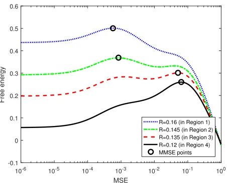
entries in the heavily marked blocks take the valuew3, except that entries along the dashed diagonal arew1. The entries in the lightly marked blocks take the valuew4, except that entries along the dotted diagonals arew2. . . 25 Figure 3.3 Free energy as a function of the MSE for different measurement ratesκ
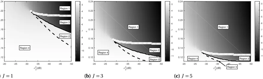
(num-ber of jointly sparse signal vectors J =3 and noise varianceσ2Z =−35 dB). The black circles mark the largest free energy, and so they correspond to the MMSE. . . 28 Figure 3.4 Performance regions for MMV with differentJ. The darkness of the shades
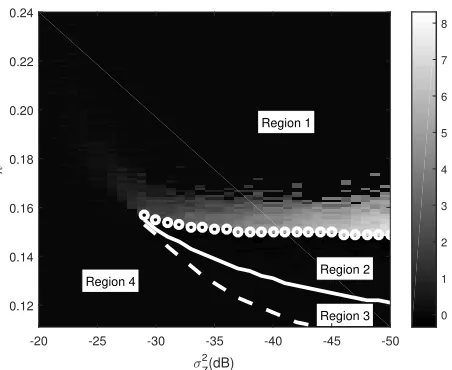
corresponds to ln(MMSE) for a certain noise varianceσZ2 and measurement rateκ. There are 4 regions, Regions 1 to 4, where the MMSE as a function of the noise varianceσZ2 and measurement rateκbehaves differently. Regions 1 to 4 are separated by 3 thresholds,κc(σ2Z)(the dashed curves),κl(σ2Z)(the solid curves), andκB P(σ2Z)(the curves comprised of little white circles); note that Section 3.5.1 discusses how to obtain these thresholds. (a) MMV with
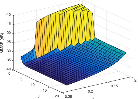
J =1, (b) MMV withJ =3, and (c) MMV withJ =5. . . 29 Figure 3.5 MMSE in dB as a function of the number of jointly sparse signal vectors J
and the measurement rateκ(noise varianceσ2
Z=−35 dB). . . 30 Figure 3.6 AMP simulation results (MSEAMP) compared to the MSE predicted for BP
(MSEBP) with J = 3 jointly sparse signal vectors. The dashed curve, solid curve, and the curve comprised of little circles correspond to thresholds
κc(σZ2),κl(σZ2), andκB P(σ2Z), respectively. Regions 1-4 are also marked. The darkness of the shades denotes lnMSEAMP
MSEBP
Figure 4.1 The optimal coding rate sequenceR∗(top panel) and optimal EMSEε∗t (bot-tom) given by DP are shown as functions oft. (Bernoulli-Gaussian signal (4.18) withρ=0.1,κ=0.4,P =100,σ2Z=4001 , andb=2.) . . . 44 Figure 4.2 Geometric interpretation of SE. In all panels, the thick solid curves correspond
togI(·)andgS(·), and their offset versionsgeI(·)andgeS(·). The solid lines with
arrows correspond to the SE of AMP. Dashed lines without arrows are auxiliary lines. Panel (a): Illustration of centralized SE. Panel (b): Zooming in to the small region just above pointS∞. Panel (c): Illustration of lossy SE. . . 45 Figure 4.3 Comparison of the additive growth rate of the optimal coding rate sequence
given by DP at low EMSE and the asymptotic additive growth rate12log2 θ1. (Bernoulli-Gaussian signal (4.18) withρ=0.2,κ=1, P =100,σ2
Z =0.01, b= 0.782.) . . . 49 Figure 4.4 Pareto optimal results provided by DP under a variety of parametersb(4.13):
(a) Pareto optimal surface, (b) Pareto optimal aggregate coding rateRa g g∗ (4.14) versus the achieved MSE for different optimal MP-AMP iterationsT, and (c) Pareto optimalRa g g∗ (4.14) versus the number of iterationsT for different optimal MSE’s. The signal is Bernoulli-Gaussian (4.18) withρ=0.1. (κ=0.4,
P =100, andσ2Z =4001 .) . . . 51 Figure 5.1 Flowchart of Algorithm 5.3 (size- and level-adaptive MCMC). L(r) denotes
running L-MCMC forr super-iterations. The parametersr1,r2,r3,r4a, andr4b are the number of super-iterations used in Stages 1 through 4, respectively. CriteriaD1−D3 are described in the text. . . 72 Figure 5.2 SLA-MCMC, EGAM, and CoSaMP estimation results for a source with i.i.d.
Bernoulli entries with non-zero probability of 3% as a function of the number of Gaussian random measurementsM for different SNR values (N=10000). . 76 Figure 5.3 SLA-MCMC and tG estimation results for a dense two-state Markov source
with non-zero entries drawn from a Rademacher (±1) distribution as a func-tion of the number of Gaussian random measurementsM for different SNR values (N=10000). . . 77 Figure 5.4 SLA-MCMC, EGAM, and CoSaMP estimation results for an i.i.d. sparse Laplace
source as a function of the number of Gaussian random measurementsM
for different SNR values (N =10000). . . 78 Figure 5.5 SLA-MCMC, tG, and CoSaMP estimation results for a two-state Markov source
with non-zero entries drawn from a uniform distributionU[0, 1]as a function of the number of Gaussian random measurementsMfor different SNR values (N =10000). . . 79 Figure 5.6 SLA-MCMC estimation results for a four-state Markov switching source as
a function of the measurement rateκfor different SNR values and signal lengths. Existing CS algorithms fail at estimating this signal, because this source is not sparse. . . 80 Figure 5.7 SLA-MCMC and EGAM estimation results for a Chirp signal as a function of
Figure 5.8 SLA-MCMC with different number of random seeds and L-MCMC estimation results for the Markov-Uniform source described in Figure 5.5 as a function of the number of Gaussian random measurementsM for different SNR values (N =10000). . . 82 Figure 5.9 AMP-UD[Ma14a; Ma16], SLA-MCMC, and tG estimation results for a dense
two-state Markov source with non-zero entries drawn from a Rademacher (±1) distribution as a function of the number of Gaussian random measure-mentsM for different SNR values (N =10000). . . 83 Figure B.1 PCC test results. The darkness of the shades shows the fraction of 100 tests
where we reject the null hypothesis (random variables being tested are un-correlated) with 5% confidence. The horizontal and vertical axes represent the quantization bin sizeγof the SQ and the scalar channel noise standard deviation (std)σpt in each processor node, respectively. Panel (a): Test the correlation betweenwtandnt. Panel (b): Test the correlation betweenwt+nt andx. . . 103 Figure B.2 Comparison of the MSE predicted by lossy SE (4.12) and the MSE of
MP-AMP simulations for various settings. The round markers represent MSE’s predicted by lossy SE, and the (red) crosses represent simulated MSE’s. Panel (a): Bernoulli-Gaussian signal. Panel (b): Mixture Gaussian signal. . . 105 Figure B.3 Justification of the discretized search space used in DP. Top panel: Empirical
PMF of the error in the cost function∆Φ{·}(·)used to verify the integrity of the linear interpolation in the discretized search space ofσ2. Bottom panel: Empirical PMF of∆Ra g g; used to verify the integrity of the choice of∆R=0.1.106 Figure B.4 Illustration of the evolution ofuet. The vertical axis showsuet =
N
CHAPTER
1
INTRODUCTION
Many problems in science and engineering can be approximated as linear, where an unknown vectorx∈RN is measured via a matrix multiplication,w=Ax, withAbeing anM×N matrix. The
measurementsyare collected afterwis corrupted by measurement noisez∈RM,
y=Ax+z. (1.1)
1.1
Linear Models and Linear Inverse Problems
1.1.1 Problem setting
There are some variants of linear models (LM’s). Based on how the measurementsyand the matrix Aare stored, we form centralized LM’s or multi-processor LM’s. We can also define linear models based on the number of underlying unknown vectorsx: if there is only one unknown vectorx, then it is a single measurement vector (SVM) problem; if there are more than one unknown vectorx, then we form a multi-measurement vector (MMV) problem.
Centralized vs. multi-processor LM’s:If the matrixAand the measurementsyin (1.1) are stored in a single processor, then we call the LM acentralized LM. Recently, there is an increasing amount of data being generated in various applications. For example, the trend of relying on Internet services and social networks is more prevalent than ever before; users of web services are generating numerous log files daily. As another example, financial analysts need to predict the changes in prices based on historical price information. Given the amount of financial derivatives and the high frequency of changes in prices, financial institutions are also overwhelmed by a vast amount of data. Another example involves recent advances in wearable devices. Health care providers can provide patients with wearable sensors that record and report the health status of patients frequently, so that the health care providers can react quickly once there is an emergency. With these ever-growing amounts of data, it is no longer practical to fit these data into a single machine, and distributed and scalable file systems such as Hadoop Distributed File Systems (HDFS)[DG08]have been developed. For the case of LM, if the matrixAand the measurementsyare so big that they have to be stored in a distributed file system such as HDFS, then we form amulti-processor (MP) LM[Mot12; Pat13; Pat14;
Han14; Han15b; Rav15; Han15a; Han16]. Consider an MP-LM withP distributedprocessor nodes
and afusion center. Each distributed processor node storesMP rows of the matrixA, and acquires the corresponding measurements of the underlying signalx. Without loss of generality, the LM in distributed processor nodep∈ {1,· · ·,P}can be written as
yi=Aix+zi,i∈
§M(p−1)
P +1,· · ·, M p
P
ª
, (1.2)
whereAi is thei-th row ofA, andyiandziare thei-th entries ofyandz, respectively.
Single measurement vector vs. multiple measurement vectors:Apart from the MP-LM, an-other type of distributed linear model involves multiple sensors. Using multiple sensors can acceler-ate the sensing speed by pointing different sensors at different regions of interest, which we call
and identically distributed (i.i.d.) noisez(j),
y(j)=A(j)x(j)+z(j), j∈ {1,· · ·,J}, (1.3) where the(j)in the super-script denotes the index of the corresponding sensor. Of particular interest in reducing the number of measurements while achieving similar signal estimation quality, distributed sensing leads to a proliferation of research on the MMV problem[CH06; Cot05; ME09; BF09], in which theJ sparse signal vectorsx(j), j∈ {1,· · ·,J}, share common non-zero supports, as explained below. Let us construct asuper-symbolxl =
xl(1),· · ·,xl(J)>, where{·}>denotes the transpose, andxl(j)is thel-th entry of the signal vectorx(j). The super-symbolsxl,l ∈ {1,· · ·,N}, follow an i.i.d. J-dimensional joint distribution,
f(xl) =ρφ(xl) + (1−ρ)δ(xl), (1.4)
whereρis thesparsity rate,φ(xl)is aJ-dimensional joint distribution, andδ(xl)is the Dirac delta function forJ-dimensional vectors. When the number of signal vectors becomes 1, i.e.,J =1, this MMV problem (1.3) becomes an SMV problem. The MMV problem has many applications such as radar array signal processing, acoustic sensing with multiple speakers, magnetic resonance imaging with multiple coils[Jun07; Jun09], and diffuse optical tomography using multiple illumination patterns[Lee11].
Linear inverse problem:Usually, estimation algorithms need to be designed to estimate the signalxgiven the matrixA, noisy measurementsy, and possible statistical knowledge about the noisez. We call this a linear inverse problem.
In this work, we focus on thelarge system limitdefined below.
Definition 1.1(Large system limit[GW08]). The signal length N scales to infinity, and the number of measurements M =M(N)depends on N and also scales to infinity, where the ratio approaches a positive constantκ,
lim N→∞
M(N)
N =κ >0.
We callκthe measurement rate.
1.1.2 Prior art and open questions
a probabilistic prior for the coefficients ofxin a known transform domain[Don10; Ran11; Ji08; SN08; Bar10]. Given a probabilistic model, some related message passing approaches learn the parameters of the signal model and achieve the minimum mean squared error (MMSE) in some settings; examples include EM-GM-AMP-MOS[VS13], turboGAMP[Zin12], and AMP-MixD[Ma14b]. As a third alternative, complexity-penalized least square methods[FN03; Don06b; HN06; HN12; RS12a]can use arbitrary prior information on the signal model and provide analytical guarantees, but are only computationally efficient for specific signal models, such as the independent-entry Laplacian model[HN06]. For example, Donoho et al.[Don06b]relies on Kolmogorov complexity, which cannot be computed[CT06; LV08]. As a fourth alternative, there exist algorithms that can formulate dictionaries that yield sparse representations for the signals of interest when a large amount of training data is available[RS12a; Aha06; Mai08; Zho12]. When the signal is non-i.i.d., existing algorithms require either prior knowledge of the probabilistic model[Zin12]or the use of training data[GO07]. In spite of the numerous algorithms to solve the linear inverse problem, there are many important gaps in the prior art, such as those listed below.
1. What is the best we can do?Along with existing algorithms for solving linear inverse problems, researchers often provide theoretic estimation accuracy guarantees for these algorithms. However, what is often missing is the optimal estimation quality associated with the linear inverse problem itself, instead of the optimal estimation quality for a specific algorithm. Such a theoretic analysis will help us evaluate the quality of each algorithm and identify the gap between a specific algorithm and the theoretically optimal estimation quality.
2. What are the costs of running an algorithm?Nowadays, due to the large amounts of data mentioned in Section 1.1.1, many systems are designed in a distributed fashion. Hence, estimation algorithms need to run in a distributed network and thus incur communication costs. There exists some work trying to save communication by designing cache systems so that each node in the network does not need to send every piece of data every time[Li15; Li16]. There are also some works using heuristics in reducing the precision of the floating-point numbers sent across the network[McM13; Tha13]. However, there is little prior art discussing the “optimal” communication scheme.
1.1.3 Contributions
In the following, we briefly discuss our contributions corresponding to each of the unsolved problems raised in Section 1.1.2. Most of our contributions are made possible by taking advantage of statistical physics tools and information theory.
1. Characterizing the optimal estimation quality:In Chapter 3, we make an analogy between the MMV problem (1.3) and a thermodynamic system and use the replica analysis[Tan02; GV05; MT06; Krz12a; Krz12b; MM09; BK15; Les15]from statistical physics to analyze the information theoretic MMSE for MMV problems with i.i.d. Gaussian measurement matrices and i.i.d. Gaussian noise. Our analysis is readily extended to other i.i.d. measurement matrices and i.i.d. measurement noise. Note that the MMSE is associated with the MMV problem (1.3) itself and is not associated with any specific estimation algorithms. Realizing that mean squared error (MSE) might not be the only metric that is of interest, we propose a future direction to extend the work of Tan and coauthors[Tan14a; Tan14b]to analyze the average error based on arbitrary user-defined error metrics for MMV problems.
2. Optimal trade-offs among different costs:In Chapter 4, we apply rate-distortion theory[CT06; Ber71; GG93; WV12a]to optimize the communication cost in a specific distributed algorithm, and propose a method to find the optimal combined cost of computation and communication. In addition, we study the asymptotic behavior of the optimal communication scheme in the limit of low excess MSE beyond the MMSE. Also, recognizing that we cannot minimize the computation cost, communication cost, and the quality of the estimate simultaneously, we study the optimal trade-offs among these different costs.
3. Designing better algorithms:In Chapter 5, we propose auniversalalgorithm that is based on the mild assumption of the signal being “simple,” i.e., there is some structure in the signal that is simple. Our algorithm is based on “simulated annealing,” a mathematical analogy to a statistical physics concept, and achieves favorable estimation accuracy while using limited prior information about the signal models. In Chapter 5, we also briefly discuss another universal algorithm that is based on belief propagation[Don09; Bar10; BM11; Mon12; Krz12a; Krz12b; BK15], which originates from statistical physics and information theory. We refer interested readers to Ma et al.[Ma14a; Ma16].
1.2
Organization, Notations, and Acronyms
1.2.1 Organization
This dissertation is organized as follows. Chapter 2 introduces some background on statistical physics and information theory. Chapter 3 studies the MMSE and its behavior for MMV problems; we also propose a future direction to study arbitrary user-defined error metrics for MMV problems. The limiting behavior of the optimal communication scheme and the optimal trade-offs among different costs in MP-LM’s are discussed in Chapter 4. In Chapter 5, we propose a universal algorithmic framework that achieves favorable estimation quality. Chapter 6 concludes the dissertation and proposes some future directions. Details about some proofs appear in the appendices.
Note that Chapter 3 is based on our work with Baron[ZB13]and with Baron and Krzakala[Zhu16b]. Chapter 4 is based on our work with Han et al.[Han16]and with Baron and Beirami[Zhu16c; Zhu16a]. Chapter 5 is based on our work with Baron and Duarte[Zhu14; Zhu15].
1.2.2 Notations
In this dissertation, bold capital letters represent matrices, bold lower case letters represent vectors, and normal font letters represent scalars. The entry (scalar) in thei-th row,j-th column of a matrixA is denoted byAi,j, where the comma is often omitted. Thei-th entry (scalar) in a vectorzis denoted byzi. Following are some frequently used notations.
• A: Measurement matrix
• C: The set of complex numbers
• D: Distortion
• δ(·): Dirac delta function
• f(·): Probability density function (continuous variable) • E[·]: Expectation
• κ: Measurement rate
• M: Number of measurements • N: Signal length
• N: The set of natural numbers, i.e.,{0, 1,· · · }
• R: Coding rate
• R: The set of real numbers
• P: Probability
• P(·): Probability mass function (discrete variable)
• ρ: Sparsity rate (percentage of non-zeros in a vector) • σ2Z: Variance of the noisez
• t: Iteration index
• A>: Transpose of matrixA • x: Signal
• kxkp:`pnorm of a vectorx; ifpis not specified, then we refer to`2norm • y: Measurements
• z: Noise
• [x1,x2,· · ·,xN]: The vector consists ofx1,x2,· · ·,xN • {1, 2,· · ·,N}: The set consists of 1, 2,· · ·,N
1.2.3 Acronyms
• AMP: Approximate message passing • BP: Belief propagation
• CS: Compressed sensing
• i.i.d.: Independent and identically distributed • LM: Linear model
• MMSE: Minimum mean squared error • MMV: Multi-measurement vector • MP: Multi-processor
• PMF: Probability mass function • RD: Rate-distortion
CHAPTER
2
STATISTICAL PHYSICS AND
INFORMATION THEORY BACKGROUND
In Chapter 1, we discussed the prior art and mentioned that our contributions are made possible by tools in statistical physics and information theory. Due to the interdisciplinary nature of this dissertation, this chapter briefly reviews some concepts and methodologies that are used in our work. We refer readers who are interested in delving into these subjects to the books by Mézard and Montanari[MM09]and by Cover and Thomas[CT06].
2.1
Relevant Statistical Physics Concepts
Statistical physics studies a disordered thermodynamic system containing a large number of parti-cles that are interacting with each other by the internal force between (among) the partiparti-cles as well as the external force applied to the entire disordered system.
2.1.1 Basics
Entropy (thermodynamics):Entropy quantifies the amount of disorder of a thermodynamic system,
S(x) =−X x
P(x)logP(x), (2.1)
where the vectorxdescribes theconfigurationof a certain thermodynamic system andP(x)is the
probability of a certain configuration existing in the disordered system. By summing over all possible configurations and accounting for their corresponding probability, we are able to obtain the level of disorder, or theentropyof this particular thermodynamic system.
Boltzmann distribution:In a thermodynamic system, the higher the temperature is, the more disordered the system is. The Boltzmann distribution is a probability distribution used to describe various possible configurations in a thermodynamic system,
P(x) =
1
Zexp
−H(x)
T
, (2.2)
where the vectorxdescribes the configuration of a thermodynamic system,T is the temperature of this system,H(x)is the energy for a certain configuration, andZ is a normalizer called thepartition function. If the thermodynamic system is in a high temperature, i.e.,T is large, then the probabilities for configurations with different energy are approximately the same and the system reaches the maximum entropy (2.1), which corresponds to the greatest amount of disorder.
Annealing and quench:The configuration associated with the lowest energy can be obtained through a process called annealing, where a disordered system gradually cools down. Intuitively, when the temperatureT decreases, the configurations with lower energy becomes more and more likely in the disordered system, according to (2.2). Given enough time that allows a slow enough decrease in the temperature, we can guarantee to obtain the globally minimum energy configuration. A related concept isquench, in which the temperature is quickly decreased, so that the disordered system is likely to achieve a local minimum energy configuration. Since the temperature is quickly decreased, once a local minimum energy configuration appears, it will be difficult to generate other lower energy configurations according to (2.2).
2.1.2 Spin glass theory basics
A basic understanding of spin glass theory provides new perspectives when solving linear inverse problems. In the following, we introduce some basics of spin glass theory. The goal is to provide intuition, and we refer interested readers to Mézard and Montanari[MM09]for rigorous and detailed explanations.
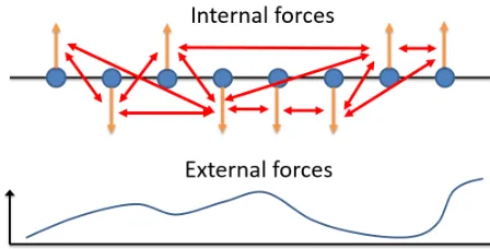
Figure 2.1 Illustration of spin glasses with internal and external forces. Each dot represents a spin glass. Vertical arrows denote the state of each glass. The remaining arrows illustrate the internal forces between pairs of spin glasses and the curve in the bottom panel illustrates the external force. Figure inspired by Ralf R. Müller.
model, there exist internal forces betweeneach pairof the spinning glasses. Moreover, we assume that there is an external force that can affect the states of the glasses. Hence, the overall energy of a specific thermodynamic system for a specificconfigurationxis
H(x) =−X i
X
j<i
ri jxixj−X i
hixi, (2.3)
wherexiis thei-th element of the configuration (vector)xand it represents the state of thei-th glass,ri j models the force between glassiand glassj, andhi models the external force applied to glassi. This model is illustrated in Figure 2.1, where each dot represents a glass, and the vertical arrows denote the state of each glass. The remaining arrows illustrate the internal forces between pairs of spin glasses and the curve in the bottom panel illustrates the external force. The energy function (2.3) is often called theHamiltonian. Note that the Hamiltonian (2.3) isquenched, because we assume thatri j andhi are constant.
One of the things that nature does is maximizing the entropy (2.1) of a thermodynamic system for a given energy (because energy is assumed to be conserved),
E=X x
P(x)H(x). (2.4)
It can be proved that the Boltzmann distribution (2.2) maximizes the entropy (2.1) for a given energy (2.4). Moreover, the energyH(x)in the Boltzmann distribution (2.2) is the Hamiltonian for configurationx(2.3).
Free energy and self-averaging:Sometimes, instead of (mathematically) evaluating the maxi-mum entropy (2.1), it is more convenient to evaluate the minimaxi-mumfree energygiven by
Using (2.1), (2.2), and (2.4) with normalization by the number of spin glassesN, we simplify (2.5) as
F =−T
N logZ, (2.6)
where the partition functionZ is the normalizer in (2.2). Note that because the Hamiltonian (2.3) is quenched, the free energy (2.6) is quenched.
The expression in (2.6) is undesirable, because we have to calculate the free energy for each of the quenched Hamiltonians. Physically, it means that we need to carry out this calculation for every specific piece of material. It turns out that when the size of the system is sufficiently large, the properties of the system do not depend on the specific settings ofri j andhiany more (2.3), which is the so-calledself-averagingproperty of a thermodynamic system, given sufficiently many particles. Hence, we define the free energy as
F=− lim N→∞
T
NE
logZ. (2.7)
2.2
Information Theory and Coding Theory
This section discusses some important results from information theory and coding theory that are relevant to this dissertation. The author refers interested readers to the book by Cover and Thomas[CT06]for further details and more comprehensive explanations. Coding theory and in-formation theory are quite related and are both widely used in digital communication systems, and we simply call them “information theory” for brevity. Seeing that information theory is widely used in digital communication systems, we start by introducing the components of a typical digital communication system. But before that, we must understand the most basic of concepts: the bit.
Figure 2.2 Illustration of a typical digital communication system. Figure inspired by Brian Hughes’ slides.
Components of a digital communication system:As illustrated in Figure 2.2, there are 7 key components of a typical digital communication system. First, the signal is encoded (compressed), so that the communication system does not need to send as many bits as required by the original signal; this step is calledsource encoding. Then, the encoded (compressed) signal is passed through a channel encoder, in which redundancy is introduced to the bit sequence. This redundancy is crucial to better utilize the energy of the transmitter and the channel. Next, the redundant sequence is modulated to an analog waveform by one of the available modulation schemes. After modulation, the transmitter sends the modulated signals (analog) through a noisy channel and the receiver receives a noisy sequence that contains the information of the original signal. Then, the receiver demodulates the noisy analog waveform into a sequence of bits. After that, the receiver decodes (channel decoder) the sequence to remove redundancy.1 Finally, with an error-free (hopefully) sequence of bits, the last step is to decompress the data.
Link between statistical physics and information theory:2In Section 2.1, we denote the config-uration of a thermodynamic system by a vectorx= [x1,· · ·,xN], wherexi,i∈ {1,· · ·,N}, represents the state of thei-th spin glass. In information theory, we typically usex= [x1,· · ·,xN]to represent a length-N signal. This signalxis passed through a channel. The counterparts of the channel in digital communication systems for statistical physics are the internal and external forces that interact with the particles of the thermodynamic system. With this brief analogy, we start introducing some important concepts and results in information theory.
Entropy (information theory):We have introduced entropy (2.1) in statistical physics. In infor-mation theory, entropy quantifies the amount of inforinfor-mation carried by a certain signalx. If the entries ofxtake discrete values, then the expression for entropy in information theory is the same as (2.1), and the only difference is thatP(x)represents the joint probability mass function of a signal
1There will be errors in the demodulated sequence. By introducing redundancy in the channel encoding step, the
channel decoder can identify and correct errors due to the noisy channel.
x. If the entries ofxare continuous, then the entropy in information theory for a signalxis
S(x) =−
Z
x
f(x)log[f(x)]dx, (2.8)
wheref(x)is the joint probability density function ofx.
Coding rate (source encoder):Before transmitting the signalx∈RN to the receiver, a
commu-nication system typically first compresses the signal, so that it can save in commucommu-nication load. The coding rate is defined as
R=Number of bits after compression
N . (2.9)
Distortion:After receiving the encoded signal,3the receiver needs to decode it. There are two types of data compression that can be used in the source encoder. One islossless compressionand the other islossy compression. In lossless compression, after the source decoder decodes the data sequence, it obtains a signal that is identical to the original signal. In lossy compression, the signal obtained after decoding is somewhat distorted from the original signal. The cause of thisdistortion
is thequantizationprocess when encoding the signal in a lossy way. A typical quantizer builds a “grid” in the space of value(s) to be quantized. Next, the quantizer rounds the value(s) to the nearest point on the grid. As an example, the scalar quantizer[GG93; CT06]rounds each (scalar) entry in the signal to the nearest grid point. The vector quantizer[Lin80; Gra84; GG93]rounds sequence of scalars to the nearest hyper-grid point.
Denote the distance between a certain entry in the original signalxi and the corresponding entry in the decoded signalxbibyd(xi,bxi), where we can use various distance functions[Kre89]for
d(·,·). The average distortion of the entire signal is given by
D= 1
N
N
X
i=1
d(xi,xbi). (2.10)
Rate-distortion theory:There is a fundamental information theoretic relation between the rate (2.9) and distortion (2.10). With a certain quantization scheme and knowledge about the distri-bution of the signal, we can calculate the coding rateR(2.9) and the expected distortionD(2.10). Although this calculation is not always an easy task[Ari72; Bla72; Ros94], a pivotal message from rate-distortion theory is that we can save a lot in the coding rateR(2.9) by allowing a small distortion
D (2.10).
Cavity method and belief propagation:We can regard the linear model in (1.1) as a communi-cation channel, wherexis the signal to be transmitted,Amodels the transmission scheme,zis the
3According to Figure 2.2, after data compression and before transmitting the sequence, there is typically a channel
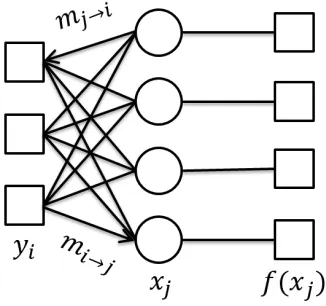
Figure 2.3 Illustration of belief propagation. The boxes are called the factor nodes and the circles are called the variable nodes.
noise in the receiver, andyis the received sequence. Belief propagation (BP)[Don09; Bar10; BM11; Mon12; Krz12a; Krz12b; BK15]is an algorithm that can be used to infer the underlying signalxin the channel (1.1). BP was invented independently by researchers in coding theory, statistical physics, and artificial intelligence. First of all, we represent the channel (1.1) as a Tanner graph in Figure 2.3, where we express each entryxj of the signalxby a variable node (circles in Figure 2.3), driven by its distributionf(xj)from a factor node (boxes in Figure 2.3). Then, variable nodes are interacting with the factor nodesyi’s.
The messagesmi→j(xj)andmj→i(xj)given by the canonical BP updating rules for the posterior distributionf(x|y)are as follows,
mi→j(xj) = 1 Zi→j
Z
Y
k6=j
mk→i(xk)
e
− 1
2σ2
Z P
k6=jAi kxk+Ai kxk−yi 2
Y
k6=j
d xk
,
mj→i(xj) = 1 Zj→i
f(xj)Y
q6=j
mq→j(xj).
(2.11)
Note that in statistical physics, the factor nodes model the forces between (or among) spin glasses (variable nodes). WhenAis sparse or locally tree-like, BP yields an estimate that converges to the true posterior distributionf(x|y). With this posterior distribution, we obtain the estimatebx=E[x|y]
CHAPTER
3
MINIMUM MEAN SQUARED ERROR FOR
MULTI-MEASUREMENT VECTOR
PROBLEM
with both real and complex measurement matrices are also analyzed. Multiple performance regions for MMV are identified where the MMSE behaves differently as a function of the noise variance and the number of measurements.
Belief propagation (BP) is a signal estimation framework for linear inverse problems that often achieves the MMSE asymptotically. A phase transition for BP is identified. This phase transition, verified by numerical results, separates the regions where BP achieves the MMSE and where it is sub-optimal. Numerical results also illustrate that more signal vectors in the jointly sparse signal ensemble lead to a better phase transition.
Realizing that the mean squared error might not be the only error metric that is of interest, we pro-pose some future directions involving the study of optimal performance for arbitrary user-defined additive error metrics for MMV problems by extending the work of Tan and coauthors[Tan14a; Tan14b].
3.1
Related Work and Contributions
In multi-measurement vector (MMV) problems, thanks to the common support, the number of sparse coefficients that can be successfully estimated increases with the number of measure-ments. This property was evaluated rigorously for noiseless measurements using`0 minimiza-tion[Dua13]. To address measurement noise, estimation approaches for MMV problems have included greedy algorithms such as SOMP[Tro06b; CH06],`1convex relaxation[Mal05; Tro06a], and M-FOCUSS[Cot05]. REduce MMV and BOost (ReMBo) has been shown to outperform conven-tional methods[ME09], and subspace methods have also been used to solve MMV problems[Lee12; Ye15]. Statistical approaches[ZS11]often achieve the oracle minimum mean squared error (MMSE). However, the performance limits of MMV signal estimation in the presence of measurement noise have not been studied.
Replica analysis is a statistical physics method that can be used to analyze the MMSE and phase transition for inverse problems[Tan02; GV05; MT06; Krz12a; Krz12b; MM09; BK15; Les15]. Barbier and Krzakala[BK15]studied the MMSE for estimating superposition codes using replica analysis. In this chapter, we extend the derivation in Barbier and Krzakala[BK15]to two related yet different MMV settings: (i) J jointly sparse signals are measured byJ different dense matrices that are independent and identically distributed (i.i.d.), and (ii)J jointly sparse signals are measured by
J identical i.i.d. matrices. We only consider dense i.i.d. Gaussian matrices in this work, while our analysis can be extended to other i.i.d. matrices easily.
with fixed length blocks. Third, we derive the MMSE for complex SMV problems by noticing that complex SMV is essentially an MMV problem. Fourth, we identify several performance regions for MMV, where the MMSE has different characteristics based on the channel noise variance and measurement rate. Finally, we find a phase transition for belief propagation algorithms (BP)[Don09; Bar10; BM11; Mon12; Krz12a; Krz12b; BK15]applied to MMV problems, which separates regions where BP achieves the MMSE asymptotically and where it is sub-optimal. BP simulation results confirm the phase transition results. Seeing that the mean squared error (MSE) might not be the only error metric that is of interest, we propose a future direction to extend the work of Tan and coauthors[Tan14a; Tan14b]to MMV settings, so that we can analyze the performance limits for arbitrary user-defined additive error metrics, as well as design an algorithmic framework that can achieve such performance limits.
The remainder of this chapter is organized as follows. We introduce our signal and measurement models in Section 3.2, followed by replica analysis for two MMV settings as well as two complex SMV problems in Section 3.3. Section 3.4 proves the results of Section 3.3. Numerical results are discussed in Section 3.5. Section 3.6 proposes some future directions to study the performance of arbitrary user-defined additive error metrics for MMV problems and we conclude in Section 3.7. Some detailed derivations appear in Appendix A.
3.2
Signal and Measurement Models
Signal model: We consider an ensemble ofJ signal vectors,x(j)∈
RN, j∈ {1,· · ·,J}, wherejis the
index of the signal. As in Section 1.1.1, we consider asuper-symbolxl =
x(l1),· · ·,xl(J)>,l∈ {1,· · ·,N}, where{·}>denotes the transpose. The super-symbolx
l follows aJ-dimensional Bernoulli-Gaussian distribution (defined in (1.4)),
f(xl) =ρφ(xl) + (1−ρ)δ(xl), (3.1) whereρis the sparsity rate,φ(xl)is aJ-dimensional Gaussian distribution with zero mean and identity covariance matrix, andδ(xl)is the delta function forJ-dimensional vectors.
Definition 3.1(Jointly sparse). Ensembles of signals that obey(3.1)are called jointly sparse.
Measurement models: Each signalx(j) is measured by an i.i.d. Gaussian measurement ma-trixA(j)∈
RM×N,A(µjl)∼ N(0,N1), whereµrefers to the row index andl is the column index. The measurementsy(j)are corrupted by i.i.d. Gaussian noisez(j)consisting of entriesz(j)
µ ∼ N(0,σ2Z), y(j)=A(j)x(j)+z(j), j∈ {1,· · ·,J}. (3.2)
this chapter is readily extended to other i.i.d. matrices, jointly sparse signals (3.1), and other i.i.d. noise distributions.
Definition 3.2(MMV-1). The setting MMV-1 refers to the measurement model in(3.2)with all matricesA(j)being different.
Definition 3.3(MMV-2). The setting MMV-2 refers to the measurement model in(3.2)with all matricesA(j)being equal.
In the signal model (3.1) and measurement model (3.2), the sparsity rate ρ, channel noise varianceσ2Z, and number of channelsJ are constant. We are interested in the large system limit, which has been defined in Definition 1.1 in Section 1.1.1. For readers’ convenience, we restate the definition of the large system limit as follows.
Definition 3.4(Large system limit[GW08]). The signal length N scales to infinity, and the number of measurements M =M(N)depends on N and also scales to infinity, where the ratio approaches a positive constantκ,
lim N→∞
M(N)
N =κ >0. (3.3)
We callκthe measurement rate.
3.3
Replica Analysis for MMV Settings
Section 3.2 discussed two MMV settings. Both settings have applications in real-world problems such as magnetic resonance imaging[Jun07; Jun09]and sensor networks[PK00]. Although numerous algorithms for MMV signal estimation have been proposed[Tro06b; CH06; Mal05; Tro06a; Cot05; ME09; ZS11], what is often missing is an information theoretic analysis of the best possible MSE performance. In this chapter, we only consider the MSE as our performance metric, except for Section 3.6.
3.3.1 Statistical physics background and replica method
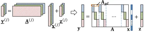
In order to express (3.2) using a single channel, we transform it to an SMV form. One possible way to do so is illustrated in Figure 3.1. The equivalent SMV problem is
y=Ax+z, (3.4)
whereA∈RM J×N J is the matrix,y∈RM J are the measurements, and the noise isz∈RM J. Entries of
Figure 3.1 Illustration of MMV channel (3.2) withJ=3 signal vectors (left), and one of its possible SMV forms (right). Different background patterns differentiate entries from different channels, and blank space denotes zeros.
x, measurementsy, and noisez(3.4) with
x(l−1)J+j =x( j)
l , y(j−1)M+µ=y( j)
µ , andz(j−1)M+µ=z( j)
µ ,
respectively. Entries of the matrixA(j)(3.2) form the SMV matrixA(3.4) withA(j−1)M+µ,(l−1)J+j =A( j)
µl; other entries ofAare zeros. The posterior for the estimatebx∈RN J, comprised of super-symbols
b
xl =
b
x(l−1)J+1,· · ·,xbl J >
, l∈ {1,· · ·,N}, is
f(bx|y) =
1
Z
N
Y
l=1
f(bxl)
M J
Y
µ=1
e−
1 2σ2
Z
yµ−PN l=1Aµlbxl
2
q
2πσZ2
, (3.5)
whereAµl = [Aµ,(l−1)J+1,· · ·,Aµ,l J]is a super-symbol highlighted by the dashed area in Figure 3.1, and the denominatorZis the partition function[Tan02; GV05; Krz12a; Krz12b; MM09; BK15],
Z=
Z
N
Y
l=1
f(bxl) M J
Y
µ=1
e−
1 2σ2
Z
yµ−PN l=1Aµlbxl
2
q
2πσ2Z
N
Y
l=1
dbxl. (3.6)
Note that multi-dimensional integrations such as (3.6) are denoted by a singleR operator for brevity. Confining our attention to the Bayesian setting[Krz12a; Krz12b; BK15],f(bxl)follows the true distribution (3.1),f(bxl) =ρφ(bxl) + (1−ρ)δ(bxl).
By creating an analogy between the channel (3.4) and a many-body thermodynamic system[Tan02; GV05; Krz12a; Krz12b; MM09; BK15], the posterior (3.5) can be interpreted as the Boltzmann measure on a disordered system with the following Hamiltonian,
H(bx) =
N
X
l=1
log[f(bxl)] +
M J
X
µ=1 1 2σ2Z
yµ− N
X
l=1 Aµlbxl
2
. (3.7)
expression provides the MMSE for the channel (3.4)[Tan02; GV05; Krz12a; Krz12b; MM09; BK15].
Under the assumption of self-averaging[Tan02; GV05; Krz12a; Krz12b; MM09; BK15], the free energy
is defined as1
F = lim N→∞
1
NEA,x,z[log(Z)], (3.8)
which is difficult to evaluate. Note thatEA,x,z[·]denotes expectation with respect to (w.r.t.)A,x, andz. The replica method[Tan02; GV05; Krz12a; Krz12b; MM09; BK15]introducesnreplicas of the estimatebxasbx
a,a ∈ {1,· · ·,n}, and the free energy (3.8) can be approximated by the replica trick[Krz12a; Krz12b; MM09; BK15],
F = lim N→∞n→lim0
EA,x,z[Zn]−1
N n . (3.9)
Note that the self-averaging property that leads to (3.8) and the replica trick (3.9), as well as the replica symmetry assumptions that appear in latter parts of this chapter, are assumed to be valid in this work, and their rigorous justification is still an open problem in mathematical physics[Tan02; GV05; Krz12a; Krz12b; MM09; BK15].2
Evaluating the free energy: To evaluate the free energy (3.9), we calculateEA,x,z[Zn]as follows,
EA,x,z
Zn= (2πσ2Z)−n M J2 ×
Ex
Z N Y
l=1 n
Y
a=1
f(bxal ) M
Y
µ=1
Xµ N
Y
l=1 n
Y
a=1
dbxal
, (3.10)
whereZis given in (3.6),
Xµ=EA,z
e−
1 2σ2
Z PJ
j=1
Pn a=1(v
a µj)2
, (3.11)
ais the replica index,bxal is thel-th super-symbol ofbxa, and
vµaj=
N
X
l=1
Aµ+M(j−1),l(xl −bx
a
l) +zµ+M(j−1). (3.12)
Lemma 3.1. In the large system limit, the quantityXµ(3.11)is the same for both MMV-1 and MMV-2. Lemma 3.1 is proved in Section 3.4. Because of Lemma 3.1, the free energy expressions for MMV-1 and MMV-2 should be identical in the large system limit. We state the result as a theorem and the detailed derivations appear in Appendix A.
1Part of the literature[Tan02; GV05], including (2.7) in this dissertation, defines the free energy as the negative of (3.8),
so that fixed points of the free energy correspond to local minima.
2Recently, the replica Gibbs free energy has been proven rigorously for the SMV case by Barbier et al.[Bar16]and
Theorem 3.1(Free energy for MMV). For settings MMV-1 and MMV-2, the free energy expressions as functions of E are identical in the large system limit and are given below,
F(E) = −J 2κ
log[2π(σ2Z+E)] +ρ+σ
2 Z
E +σ2Z
+
Z
f(x1)
Z
log
Z
f(bx1)e−
Ò Q+qb
2 bx >
1bx1+mÒbx >
1x1+
p
b
qh> b
x1d
bx1
Dhdx1 (3.13)
= −J 2κ
log[2π(σ2Z+E)] + σ
2 Z
E +σ2Z
+ J R(1−ρ) 2(κ+E+σZ2)+ ρ Z log ρ
E+σ2 Z
κ+E +σ2Z
J/2
+ (1−ρ)e−
κ
2(E+σ2
Z)
g>g
Dg+
(1−ρ)
Z
log
ρ
E+σZ2 κ+E+σ2
Z
J/2
+ (1−ρ)e−
κ
2(κ+E+σ2
Z)
h>h
Dh, (3.14)
whereh,x1, andgare J -dimensional super-symbols, and the differentialDh=
QJ
j=1 1 p
2πe −h2
j/2d h
j;
the same rule applies toDg.3
MMSE: TheE that maximizes the free energy (3.14)corresponds tothe MMSE[Krz12a; Krz12b; BK15]. After finding theE0that maximizes the free energy (3.14), we obtain the MMSE,D0=E0, in the large system limit.
Corollary 3.2. The MMSE for MMV-1 and MMV-2 is the same for the same measurement rateκ, noise varianceσ2
Z, and number of signal vectors J .
Remark 3.1. As the reader can see from the proof of Lemma 3.1 in Section 3.4, the key reason that both MMV-1 and MMV-2 have an identical MMSE is that the entries in the super-symbolsxl and
b
x{·}l are i.i.d. That said, we suspect that the MMSE for MMV-1 and MMV-2 could differ by some higher order terms. If the entries of these super-symbols are not i.i.d., which is true in some practical
MMV applications[ZS13], then it becomes more difficult to analyze the covariance matrixGµas in
Section 3.4. Therefore, we do not have an analysis for non-i.i.d. entries withinxl andbx
{·}
l . However, we
speculate that MMV-1 might have lower MMSE than MMV-2 in that case.
Link to SMV with block sparse signal:The signalxin (3.4) is a block sparse signal comprised of
N blocks of length J. We study an SMV problem by replacing the measurement matrixAin (3.4) with an i.i.d. Gaussian matrixbA∈RM J×N J, i.e.,y=Axb +z. The entries ofbAfollow the distribution,
b
Aµl ∼ N(0,N J1 ). This SMV is similar to the setting in Barbier and Krzakala[BK15], except for the different priors and different`2norms in each row ofbA. We consider these differences while following
3TheJ-dimensional integrals in (3.14) can be simplified to one-dimensional integrals using a change of coordinates
their derivation[BK15], and obtain the same free energy expression as (3.14). We have also shown that MMV-1 and MMV-2 have the same MMSE in the large system limit. Hence, the three settings have the same free energy expression and their MMSE’s are the same under the same noise variance
σ2
Z and measurement rateκin the large system limit. 3.3.2 Extension to complex SMV
The MMV model with jointly sparse signals is a versatile model that can be adapted to other problems. As an example, we show how the MMV model can be used to analyze the MMSE of a complex SMV. Consider the complex SMV,yC=ACxC+zC, wherexC=xR+ixI ∈CN,AC =AR+iAI ∈CM×N,
zC =zR+izI ∈CM,yC =yR+iyI ∈CM,i=p−1, andRandI refer to the real and imaginary parts,
respectively. The real and imaginary parts of the entries ofzC both follow a Gaussian distribution,
zlR,zlI ∼ N(0,σ2Z),l ∈ {1,· · ·,M}. Assume that the complex signalxC is comprised of two jointly sparse signals,xRandxI, that satisfy theJ =2 dimensional Bernoulli-Gaussian distribution (3.1). We can extend the analysis of Section 3.3.1 to two settings of complex SMV: (i) the measurement matrixAC is real and (ii)AC is complex.4
Real measurement matrix:Suppose thatAC is real,AC =AR∈RM×N, and the entries ofAR follow a Gaussian distribution,ARµl ∼ N(0,N1). Complex SMV with a real measurement matrix can be written as real-valued MMV,
yR=ARxR+zR andyI =ARxI+zI, (3.15)
wherexRandxI are jointly sparse and follow (3.1). This formulation (3.15) fits into MMV-2 forJ =2. Hence, we can obtain the MMSE according to (3.14).5
Complex measurement matrix: Consider a complexAC = AR +iAI ∈ CM×N with entries ARµl,AIµl ∼ N(0,21N). Expanding out the complex channel,yC =ACxC+zC, we obtain the equivalent real-valued SMV channel,
yR yI
=
AR −AI AI AR
xR xI
+
zR zI
. (3.16)
4A replica analysis for complex SMV with a real measurement matrix appears in Guo and Verdú[GV05]. Their derivation
does not cover complex matrices.
We rearrange (3.16) as follows,
yR yI
| {z }
y =
AR
:,1,−AI:,1,· · ·,AR:,N,−AI:,N AI:,1, AR:,1,· · ·,AI:,N, AR:,N
| {z }
A xR 1
x1I
.. .
xNR xNI
| {z }
x + zR zI |{z} z , (3.17)
where{:}refers to all the rows. In the rearranged channel (3.17), the measurement matrixAconsists of super-symbols,
Aµl =
¨
[ARµl,−AµIl],µ∈ {1,· · ·,M}
[AIµl,ARµl],µ∈ {M +1,· · ·, 2M} , (3.18)
and the signalxconsists ofxl =
xlR xlI
,l∈ {1,· · ·,N}. The measurements and noise arey=
yR yI and z= zR zI
, respectively. Hence,yµ=PN
l=1Aµlxl+zµ,µ∈ {1,· · ·, 2M}.
Section 3.4 shows that the free energy and MMSE for complex SMV with complex measurement matrices are the same as MMV-1 withJ =2. Note that in the free energy expression (3.14), the MSE,
D=E (A.8), is the average MSE of theJ entries ofxl. Therefore, in this complex SMV setting,D is the average MSE of the real and imaginary parts of the signal entries.
3.4
Proof of Lemma 3.1
In this section, we show that the quantityXµ(3.11) is the same for MMV-1 and MMV-2. Moreover, we show that complex SMV with a complex measurement matrix also yields the sameXµwithJ =2.
First, we rewrite (3.11) in the vector form
Xµ=Evµ
e−
1 2σ2
Z PJ
j=1
Pn a=1(vµja)2
=Evµ
e−
1 2σ2
Z
v> µvµ
, (3.19)
wherevµ= [v1 µ1,· · ·,v
a
µ1,· · ·,vµJ1 ,· · ·,vµnJ]>andvµaj is given in (3.12). In order to calculate the expec-tation w.r.t.vµin (3.19), we calculate the distribution ofvµ, which is approximated by a Gaussian distribution, due to the central limit theorem. The mean isEA,z[vµaj] =0.
We now calculate the covariance matrix,Gµ=E[vµv>µ]. The matrixGµis separated into J ×J blocks of sizen×n, as shown in Figure 3.2. The main diagonal ofGµ consists of entries w1 =


![Figure 3.1, we can see that the proof [JM12] could be extended to the MMV setting. Note that SE allows](https://thumb-us.123doks.com/thumbv2/123dok_us/1721216.1219324/45.612.92.553.85.403/figure-proof-jm-extended-mmv-setting-note-allows.webp)